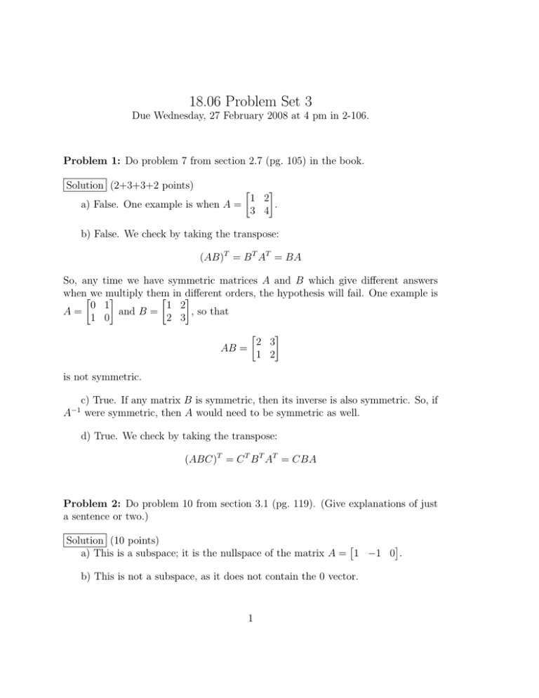
18.06 Problem Set 3
Due Wednesday, 27 February 2008 at 4 pm in 2-106.
Problem 1: Do problem 7 from section 2.7 (pg. 105) in the book.
Solution (2+3+3+2 points)
1 2
a) False. One example is when A =
.
3 4
b) False. We check by taking the transpose:
(AB)T = B T AT = BA
So, any time we have symmetric matrices A and B which give different answers
whenwe multiply
them
orders, the hypothesis will fail. One example is
in different
0 1
1 2
A=
and B =
, so that
1 0
2 3
2 3
AB =
1 2
is not symmetric.
c) True. If any matrix B is symmetric, then its inverse is also symmetric. So, if
A were symmetric, then A would need to be symmetric as well.
−1
d) True. We check by taking the transpose:
(ABC)T = C T B T AT = CBA
Problem 2: Do problem 10 from section 3.1 (pg. 119). (Give explanations of just
a sentence or two.)
Solution (10 points)
a) This is a subspace; it is the nullspace of the matrix A = 1 −1 0 .
b) This is not a subspace, as it does not contain the 0 vector.
1
c) This is not a subspace; for example, the vectors
 
 
0
1
v = 1 w = 0
1
1
both have b1 b2 b3 = 0, but their sum does not.
d) This is a subspace. Any time we take all linear combinations of a set of
vectors, we get a subspace.
e) This is a subspace; it is the nullspace of the matrix A = 1 1 1 .
f) This is not a subspace. If we take the vector
 
1
v = 2
3
and multiply it by the scalar −1, it is no longer is in the set.
Problem 3: Consider the system of equations

   
1
4
2
x1
b1
2
8
5  x2  = b2 
−1 −4 −2 x3
b3
a) For which right sides (find a condition on b1 , b2 , b3 ) is this system solvable?
b) Call the coefficient matrix A. Is the vector (2, 5, −2) in the column space of
A? How about (1, 2, 3)?
c) Suppose we add a fourth column (2, 5, −2) to A. How does the column space
change? What if we added the column (1, 2, 3) instead?
Solution (5 points)
a) We reduce the

1
2
−1
augmented matrix:



4
2 b1
1
4
2
b1
0
8
5 b2 
0
1 b2 − 2b1 
−4 −2 b3
−1 −4 −2
b3


1 4 2
b1
0 0 1 b2 − 2b1 
0 0 0 b3 + b1
2
The conditions come from the 0 rows. In this case, there is only one 0 row, giving
us the condition b1 + b3 = 0.
b) The vector (2, 5, −2) is in the column space, because b1 + b3 = 0. The second
vector is not.
c) If we append a column to A that is already in the column space, it doesn’t
change the column space. That is, we get no new linear combinations by adding
in a vector already in the space. Of course, if the column is not in C(A), then the
space gets larger.
In this case, adding (2, 5, −2) doesn’t change anything, while adding (1, 2, 3)
makes the column space equal to all of R3 .
Problem 4: Do problem 9 from section 3.2 (pg. 131).
Solution (5 points)
a) False. A counter example is a square 0 matrix (every variable is free!).
b) True. Every column is a pivot column, so there are no free variables.
c) True. There can be at most one pivot per column (because we always eliminate
so that there are 0s below each pivot).
d) True. There can be at most one pivot per row (by definition).
Problem 5: Do problem 20 from section 3.2 (pg. 132).
Solution (10 points)
We have that A is a 4 by 5 matrix, with 4 pivots. This means that only one
column can not have a pivot. Since (col 1)+(col 3)+(col 5) = 0, we know that col 5
can not have a pivot. Thus, it must be the only one without a pivot! This means
that the fifth variable is free, but the others are not.
Since there is only one free variable, there is one special solution, and the
nullspace is one-dimensional (it is exactly the scalar multiples of the special solution). The column equation tells us that the vector
 
1
0
 

v=
1
0
1
3
is in the nullspace. It is also the special solution, since x5 = 1.
Problem 6: Do problem 21 from section 3.2 (pg. 132). (Make sure the matrix you
construct has exactly the nullspace asked for in the problem, and no larger.)
Solution (10 points)
There are several ways to think about it. One way is as follows. Note that if A
is a matrix with these two vectors in its nullspace, this means that the dot product
of the first row of A with either of these vectors is 0. Switching the roles, we see
that row 1 of A must be in the nullspace of
2 2 1 0
B=
3 1 0 1
Of course, the same argument shows that every row of
of B.
So, we find the nullspace of B:
2 2 1 0
2 2
1
3 1 0 1
0 −2 − 32
A must be in the nullspace
0
1
Rescaling and putting into RR echelon form, we end up with
1 0 − 41 12
0 1 34 − 12
So, the special solutions are



1/4
−1/2
−3/4


 w =  1/2 
v=
 1 
 0 
0
1

Each row of A must be a linear combination of v and w.
Now, since A has 4 columns and exactly two independent vectors in its nullspace,
A must have rank 2. Thus, A must have at least two rows, consisting of linearly
independent combinations of v and w. Some examples would be


1/2 −3/2 2 0
1/4 −3/4 1 0
 −1
1
0 2
−1/2 1/2 0 1
0
0
0 0
4
Problem 7: a) Do problem 1 from section 3.3 (pg. 141).
b) Do problem 3 in section 3.3 (pg. 141).
Solution (5+5 points)
a) Definitions a and c are correct. Definition b is not: the identity matrix has
full rank, but b gives the answer 0. Definition d is also not correct: for example the
matrix
1 0 1
A=
0 1 1
is in row reduced echelon form and has rank 2, but has 4 ones.
b) For the original A, we obtain


1 2 0
R = 0 0 1
0 0 0
For the block matrix B, the RR echelon form is the block matrix R R . We can
see this because the row operations that reduce the left hand side A to row reduced
form will also reduce the right hand side.
The block matrix C will give us the matrix


1 2 0 0 0 0
0 0 1 0 0 0


0 0 0 1 2 0


0 0 0 0 0 1


0 0 0 0 0 0
0 0 0 0 0 0
Problem 8: Do problem 17 in section 3.3 (pg. 143).
Solution (7+3 points)
a) Suppose we can write (col j) of B in an equation
X
(col j) =
ai (col i)
i<j
We can multiply both sides of this equation on the left by A. Since matrix multiplication distributes over addition, we find that
X
A(col j) =
ai A(col i)
i<j
5
Of course, these are just the columns of AB. This shows that every free column of
B is still a free column of AB, i.e. rk(AB) ≤ rk(B). Note that left multiplying by
A can actually introduce new relations between the columns, so that the rank can
go down. We’ll see an example in part b.
1 1
b) We have B =
. If A1 is the identity matrix, then rk(A1 B) = rk(B) = 1.
1 1
If A2 is the 0 matrix, then rk(A2 B) = rk(0) = 0.
Problem 9: Define the matrix

1
1
A=
0
0
2
2
0
0
2
3
1
1
4
6
2
1

6
9

3
0
a) Reduce A to ordinary echelon form. What are the pivots? What are the free
variables?
b) Find a special solution for each free variable. (Set the free variable to 1. Set
the other variables to 0.)
c) By combining the special solutions, describe every solution to Ax = 0.
d) What is the rank of A? Which columns will generate the column space C(A)?
Solution (3+2+2+3 points)
a) We reduce:

1 2 2
1 2 3

0 0 1
0 0 1
4
6
2
1

6
9

3
0

1
0

0
0

1
0

0
0

1
0

0
0
2
1
1
1
4
2
2
1
2
0
0
0
2
1
0
1
4
2
0
1
2
0
0
0

2 4
6
1 2
3

0 −1 −3
0 0
0
Columns 1,3,4 are pivots, and columns 2,5 are free.
6

6
3

3
0

6
3

0
0
2
0
0
0
b) The special solutions are:
x2 = 1, x5 = 0 leads to (−2, 1, 0, 0, 0).
x2 = 0, x5 = 1 leads to (0, 0, 3, −3, 1).
c) The nullspace is all linear combinations of the special solutions.
d) The rank of A is 3 (the number of pivots), and these columns (1,3,4) generate
the column space.
Problem 10: Do problem 4 in section 3.4 (pg. 152).
Solution (10 points)
We first find a particular solution by reducing the augmented matrix:




1 3 1 2 1
1 3 1 2 1
2 6 4 8 3
0 0 2 4 1
0 0 2 4 1
0 0 2 4 1


1 3 1 2 1
0 0 2 4 1
0 0 0 0 0
The reduction of A has two pivots (columns 1 and 3) and two free variables (columns
2 and 4). To find a particular solution, we set the free variables to 0 and solve
U x = (1, 1, 0). Setting x2 = x4 = 0 implies x1 = 1/2 and x3 = 1/2. (Of course there
are other particular solutions; we just need to find one by setting the free variables
to whatever we like. 0 is an easy choice.)
Now, we find the nullspace of A using special solutions. We’ve already done the
work to reduce A, so we forget about the augmented part and solve U x = 0. We
find:
x2 = 1, x4 = 0 implies x1 = −3 and x3 = 0.
x2 = 0, x4 = 1 implies x1 = 0 and x3 = −2.
The complete solution is the particular solution plus all the vectors in the
nullspace:
 
 
 
−3
0
1/2
0
 0 
1
 
 

x = xp + xn = 
1/2 + c1  0  + c2 −2
0
1
0
for any choice of c1 and c2 .
7
Problem 11: Do problem 21 in section 3.4 (pg. 154).
Solution (5+5 points)
a) Here A = 1 1 1 . It has one pivot and two free variables. We find a
particular solution by setting the free variables to 0 and solving U x = 4: we get
 
4

xp = 0
0
The special solutions are found by setting one free variable to 1, one to 0, and solving
U x = 0. We find special solutions
   
−1
−1
1 0
0
1
Thus
 
 
 
4
−1
−1





xp + xn = 0 + c1 1 + c2 0 
0
0
1
for any choice of c1 and c2 .
b) We augment and reduce to get
1 1 1 4
0 −2 0 0
4
So, a particular solution is found by setting x3 = 0 and solving U x =
, thus
0
x1 = 4 and x2 = 0. The nullspace is found by setting the free variable to 1 and
solving U x = 0. In sum we get
 
 
4
−1



xp + xn = 0 + c1 0 
0
1
for any choice of c1 .
8