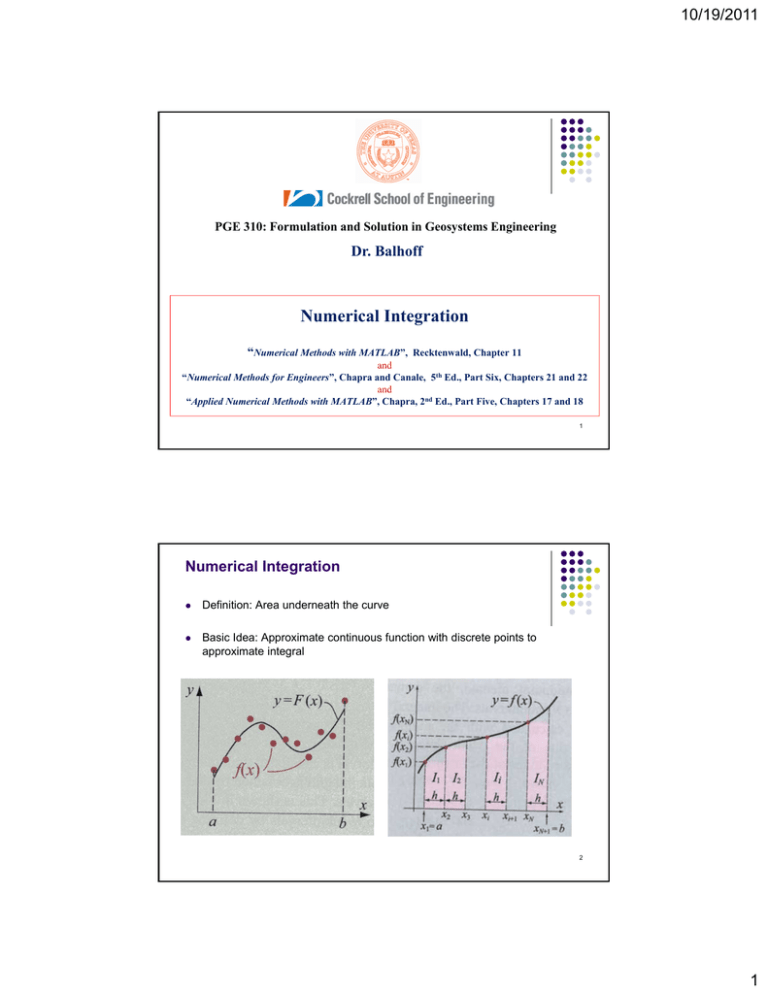
10/19/2011
PGE 310: Formulation and Solution in Geosystems Engineering
Dr. Balhoff
Numerical Integration
“Numerical Methods with MATLAB”,
Recktenwald, Chapter 11
and
“Numerical Methods for Engineers”, Chapra and Canale, 5th Ed., Part Six, Chapters 21 and 22
and
“Applied Numerical Methods with MATLAB”, Chapra, 2nd Ed., Part Five, Chapters 17 and 18
1
Numerical Integration

Definition: Area underneath the curve

Basic Idea: Approximate continuous function with discrete points to
approximate integral
2
1
10/19/2011
Methods for Numerical Integration

Curve-Fitting



Newton-Coates





Fit a curve to the discrete data
Analytically integrate curve
Complicated function or tabulated data
Replace with approximating function that is easy to integrate
Single function OR piecewise polynomials can be used
Trapezoidal, Simpson’s rules
Other methods where the function is given

Gauss quadrature Integration
3
Newton-Coates Integration Examples
Integration by (a) single straight line and (b) parabola
4
2
10/19/2011
Trapezoidal Rule – Simplest Newton-Coates
5
Integral is the Area under the Curve
Width  b  a
I  (b  a)
H 1  f (a)
f ( a)  f (b)
2
H 2  f (b )
6
3
10/19/2011
Trapezoidal Rule

First of the Newton-Coates formulas; corresponds to 1st order
polynomial
b
b
a
a
I   f ( x ) dx   f1 ( x ) dx

Recall from “INTERPOLATION” that a straight line can be represented:
f1 ( x)  f (a ) 

Area under line is an estimate of the integral b/w the limits “a” and “b”
b
I   [ f (a ) 
a

f (b)  f (a )
x
ba
f (b)  f (a)
x] dx
ba
Result of the integration is called the trapezoidal rule
I  (b  a)
f ( a)  f (b)
2
7
Error of the Trapezoidal Rule

Straight line segment to approximate integral results in error (which may be
substantial)
Et  
1
f ( )(b  a ) 3
12
or
Et  
(b  a )3
f ( )
12
Constant
a< <b
Second derivation of the function at a
point in between a and b
4
10/19/2011
What does this error mean?
y
Et  k f ( )
f(x) is a line (1st order)
f ( )  0
Zero for all  : a <  < b
x
y
Error of using Trapezoidal method = 0
It is exact.
f(x) is 2nd order
f ( )  const ant
Constant for all  : a <  < b
Error of using Trapezoidal method is
a constant value.
x
y
f(x) is a 3rd order or higher
f’’( is not constant.
f’’( is a function of 1st or higher order.
The value of f’’( changes for different
functions and different . ( a <  < b)
x
Error of using Trapezoidal method for 3rd or higher order
functions changes from case to case.
Multiple Application Trapezoidal Rule



Improve accuracy by using multiple segments
n+1 equally spaced data, so n segments of equal width
ba
h
n
The total integral can be represented by:
I
x2

x1
x3
xn1
x2
xn
f1 ( x)dx   f 2 ( x)dx   

f n ( x)dx

Substituting the trapezoidal rule yields

f ( x2 )  f ( x3 )
f ( xn )  f ( xn 1 )
f ( x1 )  f ( x2 )
h
  h
2
2
2
Grouping terms:
I h
n
f ( x1 )  2 f ( xi )  f ( xn 1 )
n
h

I  b  a 
  f ( x1 )  2 f ( xi )  f ( xn 1 ) 
 
2n
i2


 2
i2
Width
10
Average Height
5
10/19/2011
Simpson’s Rules

Higher-order polynomials another way to get more accurate estimate

Three points make a parabola, 4 points make a cubic
11
Simpson’s 1/3 Rule
b
b
a
a
I   f ( x)dx   f 2 ( x)dx

Second-order Lagrange polynomial, in the integral becomes
x3
  x  x2  x  x3 
 x  x1  x  x3  f x   x  x1  x  x2  f x dx
I  
f ( x1 ) 
 
 
x  x2  x1  x3 
 x2  x1  x3  x2  2  x3  x1  x3  x2  3 
x1   1

After the integration and algebraic manipulation:
I
f ( x1 )  4 f ( x2 )  f ( x3 )
h
 a
 f ( x1 )  4 f ( x2 )  f ( x3 )  b
 
3
6


width
Average
Height
12
6
10/19/2011
Error estimate of Simpson’s 1/3 rule

Single segment application of Simpson’s 1/3 rule has truncation
error:
Et 
1 5 (4)
(b  a )5 (4)
h f ( )  
f ( )
90
2880
4th derivation of the function at a point in
between a and b
Constant

Simpson’s rule is more accurate than the trapezoidal rule

It’s actually more accurate than expected:


Expect proportional to third derivative, but instead is proportional to
the 4th derivative
Yields an exact result for cubic polynomials even though its derived
from a parabola!
Error in Simpson’s 1/3 rule
y
Et  m f ( 4) ( )
f(x) is from 1st order to 3rd order
f ( 4 ) ( )  0
x
y
a< <b
Error of using Simpson’s 1/3 method = 0
It is exact.
Zero for all  : a <  < b
f(x) is 4th order
f ( 4 ) ( )  const ant
Constant for all  : a <  < b
Error of using Simpson’s 1/3 method
is a constant value.
x
y
f(x) is a 5th order or higher
f’’( is not constant.
f’’( is a function of 1st or higher order.
The value of f’’( changes for different
functions and different . ( a <  < b)
x
Error of using Simpson’s 1/3 method for 5th or higher order
functions changes from case to case.
7
10/19/2011
Multiple Application 1/3 Rule
h
ba
n

n segments of equal width

Total integral can be represented by:
I
x2

x1

xn1
x2
xn

f n ( x)dx
Substituting the Simpson’s 1/3 rule yields
I  2h

x3
f1 ( x)dx   f 2 ( x)dx   
f ( x1 )  4 f ( x2 )  f ( x3 )
f ( x3 )  4 f ( x4 )  f ( x5 )
f ( xn 1 )  4 f ( xn )  f ( xn 1 )
 2h
   2h
6
6
6
Grouping terms
f ( x1 )  4
n

f ( xi )  2
n 1

f ( x j )  f ( xn 1 )
n
n 1

h
  f ( x1 )  4  f ( xi )  2  f ( x j )  f ( xn 1 ) 
I  b  a 
 
3n
3
i

2,4,6
j

3,5,7



Width
i  2,4,6
j 3,5,7
Average Height
15
16
8
10/19/2011
Simpson’s 3/8 Rule
b
b
a
a
I   f ( x)dx   f3 ( x) dx

I
Integration and algebraic manipulation of the Lagrange Polynomials:
f ( x1 )  3 f ( x2 )  3 f ( x3 )  f ( x4 )
3h
 f ( x1 )  3 f ( x2 )  3 f ( x3 )  f  x4     b  a 
 
8
8


width

Average
Height
Error:


Same order accuracy as Simpson’ 1/3 rule – so 1/3 rule is usually desired
Sometimes combine 1/3 and 3/8 rule when the segments are odd
Et 
3 5 (4)
(b  a )5 (4)
h f ( )  
f ( )
80
6480
17
Integration with Unequal Segments

Until now all formulas have been based on equally spaced data

In practice, there are many situations where this does not hold

Trapezoid rule for example:
I  h1

f ( x2 )  f ( x3 )
f ( xn )  f ( xn 1 )
f ( x1 )  f ( x2 )
 h2
   hn
2
2
2
Program can easily be created to accommodate unequal sized
segments
18
9
10/19/2011
Use of the Trapezoidal rule to determine the integral of unevenly spaced data.
Notice how the shaded segments could be evaluated with Simpson’s rule to attain
19
higher accuracy
Comparison of Methods
Method
b
b
a
a
I   f ( x)dx   f1 ( x)dx
Equation
(b  a)
Trapezoid
Error
f  x1   f  x2 
2
Et  
1
3
f "  b  a 
12
n
(b  a )
1/3 Simpson’s
Rule
(b  a )
f  x1   2 f  xi   f  xn 1 
3/8 Simpson’s
Rule
2n
f  x1   4 f  x2   f  x3 
6
f  x1   4
(b  a )
Ea  
i2
Et  
i
j  3,5,7
j
n 1
3n
f  x1   3 f  x2   3 f  x3   f  x4 
(b  a )
8
2880
Ea  
Et  
12n
3
b  a 5
n 1
n
 f x  2  f x  f x 
i  2,4,6
b  a 3
b  a 5
180n
4
b  a 
6480
5
n

 f"
i 1
f ( 4 )  
n
 ( 4)
f
i 1
f (4)  
20
10
10/19/2011
Higher Order Newton-Coates
* To keep consistent notation in the above table replace x0 with x1, x1 with
x2, etc.
21
True Percent Relative Error
22
11
10/19/2011
Gauss Quadrature

Newton-Coates uses predetermined or fixed base points

Suppose we could evaluate the area under a straight line joining any
two points on the curve


We could balance the positive and negative errors if chosen wisely
Gauss Quadrature: class of techniques that implements this strategy

Particular Formulas discussed here a Gauss Legendre
Trapezoidal Rule
Gauss Quadrature
23
Method of Undetermined Coefficients:
2-Point Gauss-Legendre
• This is another approach for calculating integrals. Not using before-mentioned
methods such as Trapezoidal and Simpsons.
• In this method, for whatever function it is the integral expressed as:
y
Constant Coefficients
I  c1 f ( x1 )  c2 f ( x2 )
Value of the function at two indicative
points within the interval
a <x1 & x2 < b
a x1
x2 b
x
• So, the question is what are these 4 unknowns (c1, c2, x1 & x2) such that:
b
I   f ( x )dx  c1 f ( x1 )  c2 f ( x2 )
a
12
10/19/2011
Solve it for a Special Case:

What special?
 Want to have exact solution for any 3rd order function
 Integral limits are -1 to +1

We solve for this special case and generalize it
General 3rd order
function
g ( x)  a0  a1 x  a2 x 2  a3 x 3
1
1
1
1
I   g ( x )dx   (a0  a1 x  a2 x 2  a3 x 3 )dx
1
1
1
1
1
1
1
1
 a0  1 dx  a1  x dx  a2  x 2 dx  a3  x 3 dx
So, if the Gauss-Quadrature formula (c1x1+c2x2) can calculate exact solution for
these 4 components, it can find exact solution for the whole function.
Solve it for a Special Case:

If f(x)=1:

1
1


1

1
1

1
1

x2
x1
x12
0  c1  x1  c2  x2
x22
2
2
2
 c1  x1  c2  x2
3
x 2 dx  c1 f ( x1 )  c2 f ( x2 )
If f(x)=x3:

2  c1  1  c2  1
x dx  c1 f ( x1 )  c2 f ( x2 )
If f(x)=x2:

1
1 dx  c1 f ( x1 )  c2 f ( x2 )
If f(x)=x:
1
1
x13
x23
x 3 dx  c1 f ( x1 )  c2 f ( x2 )
4 Equations and 4 unknowns:
When solved:
3
0  c1  x1  c2  x2
c1  1
x1 
3
c2  1
1
 0.5773503
3
x2 
1
 0.5773503
3
13
10/19/2011
Method of Undetermined Coefficients:
2-Point Gauss-Legendre
y
f(x)=1
• So, we found two points (x1=-0.5773503 &
x2=+0.5773503) and two constants (c1=1 & c2=1)
such that they can return Exact Integral Value for
these four functions.
-1
x1
x
x2 +1
y
f(x)=x
-1 x1

1
1
x
x2 +1
For these four functions:
y
f ( x ) dx  c1 f ( x1 )  c2 f ( x2 )
 1 f ( 
1
1
)  1 f ( 
)
3
3
f(x)=x2
x
x2 +1
-1 x1
y
f(x)=x3
-1 x1
x
x2 +1
Method of Undetermined Coefficients:
2-Point Gauss-Legendre
• Any general 3rd order function composed of the four mentioned functions (go back to
two last slide).
• So, by using 2-Point Gauss-Legendre method we can find the Exact Solution for the integral of
any 3rd function:
For these any 3rd (or lower) order functions:

1
1
f ( x) dx  c1 f ( x1 )  c2 f ( x2 )  1 f (
1
1
)  1 f ( 
)
3
3
• For any higher order (4th order or higher) polynomial, or any non-polynomial function 2-Point
Gauss-Legendre method does not return the Exact Solution. It will have some errors and returns
Approximate Solution.
14
10/19/2011
Method of Undetermined Coefficients:
Multiple-Point Gauss-Legendre
• We can use even more points
In general form:
n-Point Gauss-Legendre formula:
Method

1
1
f ( x ) dx  c1 f ( x1 )  c2 f ( x2 )  ...  cn f ( xn )
Exact answer for functions:
Error on the order of :
3rd
2-Point Gauss-Legendre
3-Point Gauss-Legendre
4-Point Gauss-Legendre
….
n-Point Gauss-Legendre
~f(4)()
~f(6)()
~f(8)()
….
~f(2n)()
up to
order
up to 5th order
up to 7th order
….
up to (2n-1)th order
What about the Integration Limits?

Integration limits: -1 to 1; change of variables can be made to translate the
limits of integration from “a” to “b”

Introduce new variable xd related to original variable x in a linear fashion
x  a0  a1 xd

Limits: x = a and x = b corresponds to xd=-1 and xd=1
a  a0  a1 (1)

Equations can be solved simultaneously for:
a0 

b  a0  a1 (1)
ba
2
a1 
ba
2
They can substituted into equation and differentiated to yield:
x
b  a   b  a xd
2
dx 
b  a  dx
2
d
15
10/19/2011
General Form of Using Gauss-Quadrature Method Using
Higher-Point Formulas

b
a
g(xd)
ba
f ( x) dx   f (a0  a1 xd ) (
)dxd
1
2
1
  g ( xd )dxd  c1 g ( xd 1 )  c2 g ( xd 2 )  ...  cn g ( xdn )
1
1
xd i
Error:
~f 4()
~f 6()
~f 8()
~f 10()
~f 12()
In summary

Numerical Integration necessary for discrete data, complicated functions, etc.

Newton-Coates (good for predetermined and/or equally spaced data)




Trapezoid Rule (1st order accurate i.e. 2nd derivative error)
Simpson’s 1/3 (3rd order accurate i.e. 4th derivative error)
Simpson’s 3/8 (3rd order accurate i.e. 4th derivative error)
Gauss Quadrature/Gauss Legendre



More accurate, but requires us to be able to evaluate function at specific points
2-point Legendre is 3rd order accurate (Truncation error is proportional to 4th derivative)
Higher-Point Formulas Available
32
16