The Lorenz Equations
The Lorenz attractor arises in a simplified system of equations describing
the two-dimensional flow of fluid with uniform depth and imposed temperature difference between the upper and lower surfaces.
Temperature : T 1
H
x is proportional to the intensity of convection motion.
y is proportional to the temperature difference between the ascending and
descending currents.
z is proportional to the distortion of the vertical temperature profile from linearity.
Temperature : T 2
ΔT = T 1 − T 2 = constant
The meaning of parameters in the Lorenz equations
„
„
„
„
sigma is called the Prandtl Number: the ratio of
momentum diffusivity (Kinematic viscosity) and thermal
diffusivity.
r is called the Rayleigh Number: determine whether the
heat transfer is primarily in the form of conduction or
convection.
b is a geometric factor.
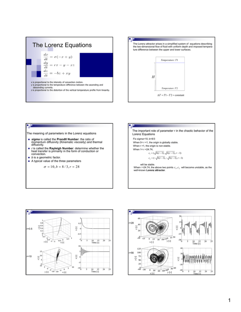
A typical value of the three parameters
The important role of parameter r in the chaotic behavior of the
Lorenz Equations
Fix sigma=10, b=8/3
When 0< r <1, the origin is globally stable.
When r >1, the origin is non-stable.
When 1< r <24.74,
c1 = ( b ( r − 1), b ( r − 1), r − 1)
c2 = ( − b(r − 1), − b(r − 1), r − 1)
will be stable.
When r >24.74, the above two points c1 , c2 will become unstable, as the
well-known Lorenz attractor.
σ = 10, b = 8 / 3, r = 28
r=28
r=0.5
r=56
r=10
1
Assume the Lorenz equations is the weather we want to predict.
Question: How confident we are???
Answer: Certainly NOT 100%
Reasons: Because the initial condition and model parameters are
imperfectly known by the predictors.
y construction probabilistic
p
models of dynamical
y
systems,
y
,
Solution: by
one of them is the parametric probabilistic approach.
Parametric probabilistic models incorporate uncertainty by modeling
certain parameters and initial condition of a prediction model by random
variables. In this case, the output of the probabilistic model will also be
random variables. The mean values of the output random variables is
often interpreted as the best estimates, while the standard deviations
can be viewed as a measure of the uncertainty in the prediction.
A parametric probabilistic model of the Lorenz equations.
dx
(t , a ) = σ ( a )(− x(t , a ) + y (t , a))
dt
dy
(t , a ) = r (a ) x(t , a ) − y (t , a ) − x(t , a ) z (t , a )
dt
dz
(t , a ) = −b( a ) z (t , a ) + x(t , a) y (t , a )
dt
A fundamental problem (in the practical construction):
The choice of the probability density functions of the random variables.
For convenience of computation, we simply choose uniform distribution.
Computation with the probabilistic model
Fix sigma=10, r=28, and b=8/3.
Step 1: choose a time step Δ t and a number n T of total time steps.
choose a number n sof Monte Carlo samples.
Step 2: simulate a set {xs , ys , zs 1 ≤ s ≤ ns } of
independent and identically distributed samples of random variables x 0 , y 0 , z 0 .
0
0
0
Step 3: for each 1 ≤ s ≤ ns, solve the deterministic Lorenz equations with
0
0
0
the initial condition xs , ys , z s , using first-order Euler time stepping
algorithm
t=0.5
Statistical mean of the
samples of x(t,a)
At t =0.5, t=5 and t = 25
as a function of the number of
Monte Carlo samples
t=5
t=25
Step 4: statistical estimation of quantities, like mean value and standard
deviation, etc.
Now, choose Δt = 0.01 and nT = 2500 .
Mean and standard deviation of x(t,a) as function of time.
All results to follow have been obtained with n s = 10, 000
Contours of the joint probability density function of x(t,a) and y(t,a)
t=5
Mean
t=25
Standard deviation
2
This figure shows the large sensitivity of the response of the Lorenz system
to small uncertainties in the initial conditions.
Fix sigma=10, b=8/3 as before, but let r be a random and
time-depend quantity, r (t , a ) = r0 + s ( a )(t − t0 ) with r0 = 28, t0 = 0
s(a)is a uniform random variable taking values in the interval
[0, (56-28)/2500].
From now on, we try to predicting the absolute value of x. Let
D ( t , a ) = x ( t , a ) and decompose it as
l (t , a )
D (t , a ) = D (t , a ) + D
where:
D (t , a ) =
1
2h
∫
t+h
t−h
D ( s , a ) ds
D(t , a) a slowly varying moving-average component.
l ( t , a ) is a fast varying component.
D
95%-confidence regions for x(t,a) as a function of time
Here the total time steps
nT = 25, 000 not 2500 as we chosen before
D(t , a)
D (t , a )
We choose
l (t , a) as a
95%-confidence regions for D(t , a ) and D
function of time.
l (t , a )
D
h = 10 here.
We can observe D(t , a) is much less sensitive to the uncertainty introduced
l (t , a) , suggesting the slow component of the response
in the model than D
can be predicted with good accuracy, whereas the fast component cannot.
From a climate change perspective, we may consider r as the CO2
concentration in the atmosphere: we know that it is increasing, but we don’t
know by how much. And its increasing rate is highly dependent on the
decision we made in future. So when we try to predict weather or climate a
random
d
variable
i bl may b
be a b
better
tt choice.
h i
Furthermore we may view the slow component as the climate response and
the fast component as the weather response. The results obtained above
Illustrate that accurate long-term predictions may be feasible for the climate,
even when they are not for the weather.
3
Predict regime changes in Lorenz model: result from RISE
(Research Internships in Science and Engineering) program at University
of Maryland, summer 2002
Imaging that you are a forecaster living the Lorenz attractor. We know there
are two different weather regimes, which we could denote as ‘warm’ and
‘cold’.
Question: can you develop simple forecasting rules to predict when changes
i regime
in
i
will
ill happen
h
and
d how
h
long
l
will
ill they
th llast?
t?
A simple method: Bred Vector
Definition: Bred Vector is the periodically rescaled difference between two
model runs, the second originating from slightly perturbed initial conditions.
First model: the real weather
Second model: people’s predict
red points means growth rate >1.8 in 8 steps.
4