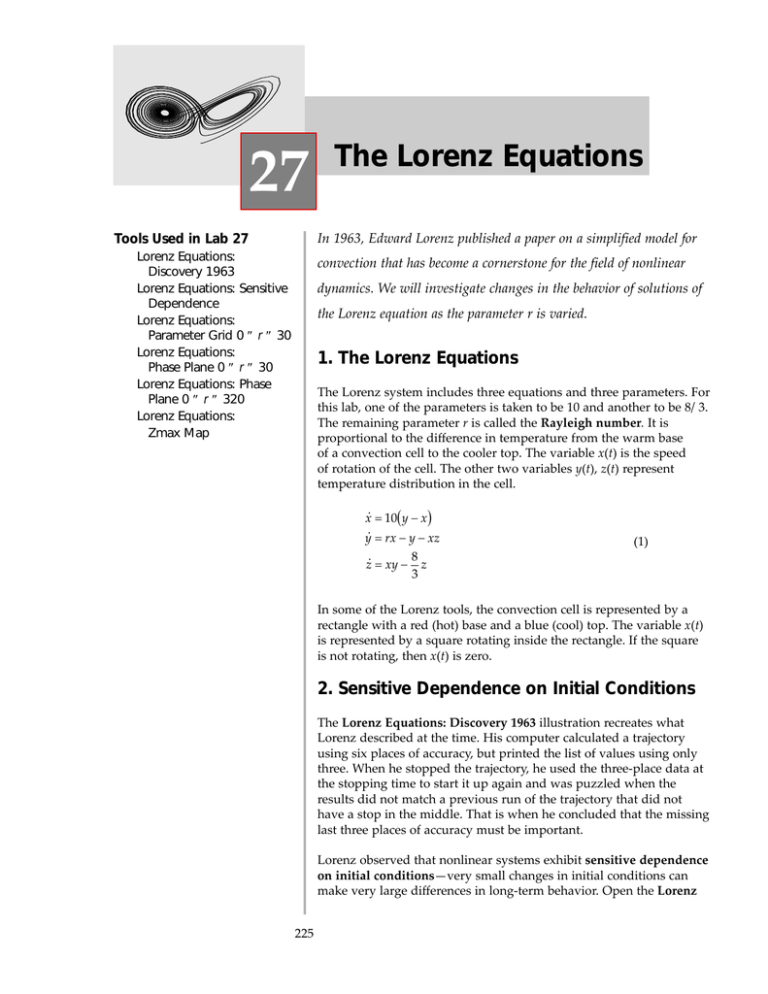
527
The Lorenz Equations
In 1963, Edward Lorenz published a paper on a simplified model for
Tools Used in Lab 27
Lorenz Equations:
Discovery 1963
Lorenz Equations: Sensitive
Dependence
Lorenz Equations:
Parameter Grid 0 ≤ r ≤ 30
Lorenz Equations:
Phase Plane 0 ≤ r ≤ 30
Lorenz Equations: Phase
Plane 0 ≤ r ≤ 320
Lorenz Equations:
Zmax Map
convection that has become a cornerstone for the field of nonlinear
dynamics. We will investigate changes in the behavior of solutions of
the Lorenz equation as the parameter r is varied.
1. The Lorenz Equations
The Lorenz system includes three equations and three parameters. For
this lab, one of the parameters is taken to be 10 and another to be 8/3.
The remaining parameter r is called the Rayleigh number. It is
proportional to the difference in temperature from the warm base
of a convection cell to the cooler top. The variable x(t) is the speed
of rotation of the cell. The other two variables y(t), z(t) represent
temperature distribution in the cell.
x˙ = 10( y − x )
y˙ = rx − y − xz
8
z˙ = xy − z
3
(1)
In some of the Lorenz tools, the convection cell is represented by a
rectangle with a red (hot) base and a blue (cool) top. The variable x(t)
is represented by a square rotating inside the rectangle. If the square
is not rotating, then x(t) is zero.
2. Sensitive Dependence on Initial Conditions
The Lorenz Equations: Discovery 1963 illustration recreates what
Lorenz described at the time. His computer calculated a trajectory
using six places of accuracy, but printed the list of values using only
three. When he stopped the trajectory, he used the three-place data at
the stopping time to start it up again and was puzzled when the
results did not match a previous run of the trajectory that did not
have a stop in the middle. That is when he concluded that the missing
last three places of accuracy must be important.
Lorenz observed that nonlinear systems exhibit sensitive dependence
on initial conditions—very small changes in initial conditions can
make very large differences in long-term behavior. Open the Lorenz
225
226
Interactive Differential Equations
Equations: Sensitive Dependence tool for an illustration of sensitive dependence on initial conditions for
the trajectory (x(t),y(t),z(t)) when r = 28. Note also that any trajectory, when r = 28, approaches a strange
attractor, that is, an attractor that is not an equilibrium, nor a cycle, nor a finite graph.
3. Equilibria of the Lorenz System
The origin is an equilibrium of the Lorenz equation.
3.1
Linearize the equations in Equation (1) at the origin. Find the eigenvalues of the linearized system
and show that the origin is an attractor for the linearized system if r < 1, but is unstable if r > 1.
. All eigenvalues will have negative real part if r < 1.
3.2
Show, in fact, that for r < 1, every trajectory is asymptotic to the origin by showing that
E( x , y , z) =
x2
+ y 2 + z 2 is a Lyapunov function for the Lorenz equation. That is, show that
10
d
E( x(t), y(t), z(t)) < 0 if r<1 and ( x , y , z) ≠ (0, 0, 0) .
dt
This last expression is strictly negative if r < 1 and (x, y, z) ≠ (0, 0, 0).
3.3
Solve the Lorenz equations with initial conditions (x(0), y(0), z(0)) = (0, 0, z0) and show that for every
value of r, every point on the z-axis is attracted to the origin.
If x = y = 0, the Lorenz equations reduce to
these have as a solution
3.4
With the given initial conditions,
.
Show that the Lorenz equations are symmetric with respect to the z-axis.
The Lorenz equations are left unchanged by the change of variables
.
For r > 1, the Lorenz equation has two additional equilibria, C+ and C–. These two points lie at the center
of each of the two “butterfly wings” comprising the strange attractor when r = 28.
Lab 27
Lorenz Equation
3.5
Find formulas for C+ and C–.
3.6
Linearize Equation (1) at C+.
227
The characteristic equation for the linear equation in Exercise 3.6 is:
λ3 +
41 2  8
80 
160
λ +  r + λ +
(r − 1) = 0
3
3
3
3
For r > 0, this equation has solutions λ 0 < 0 and a ± bi . Thus, if a < 0, C+ is an attractor and if a > 0, C+ is a
repellor. The point C+ changes from attractor to repellor at a value of r for which a = 0. The characteristic
equation then has the form:
(λ − λ0 )(λ − bi)(λ + bi) = (λ − λ0 )(λ2 + b 2 ) = λ3 − λ0 λ2 + b 2 λ − λ0b 2 = 0
3.7
By comparing coefficients of the two forms of the characteristic equation, we get three equations in
the three unknowns λ0, b, r. Solve for r to get the value of r at which C+ and C– turn from attractor to
repellor.
Comparing coefficients gives the three equations:
These can be solved to give r = 24.74.
We have seen that the origin is an attractor for r < 1. As r increases, a bifurcation occurs at r = 1. For r >1,
the origin becomes an unstable equilibrium and two attracting equilibria, C+ and C–, are born. At r = 24.74,
C+ and C– become unstable. The origin, C+ and C– are the only equilibria. Thus for r > 24.74 there are no
attracting equilibria. However, chaotic behavior already begins at r = 24.06.
For a fixed value of the parameter r, there is a large ellipsoidal trapping region for the Lorenz equation
such that all trajectories enter that region and none leave. See, for example, Exercise 9.22, p. 343 of
Nonlinear Dynamics and Chaos, by Steven H. Strogatz. Thus within that region, there must be an attractor: a
point, a cycle, or a strange attractor.
Use the Lorenz Equations: Parameter Grid 0 ≤ r ≤ 30 tool and the Lorenz Equations: Phase Plane
0 ≤ r ≤ 30 tool to verify the asymptotic behavior of solution curves for various values of r we have
described up to this point.
228
Interactive Differential Equations
4. Other Types of Behavior
Nonlinear systems, which exhibit chaotic behavior for certain choices of parameters, exhibit a variety of
interesting behaviors. Open the Lorenz Equations: Phase Plane 0 ≤ r ≤ 320 tool to explore the ideas in this
section.
Transient Chaos: Chaotic behavior begins when r = 24.06. When r ≤ 24.06, all trajectories approach an
equilibrium. For values of r less than 24.06, but close to 24.06 and for some choices of initial conditions,
trajectories will appear to be chaotic for an interval of time before approaching the equilibrium. This
phenomenon is called transient chaos.
Periodic Windows: Even though for many choices of parameter r > 24.74, the behavior of the system is
chaotic, there are intervals of parameters on which the trajectories approach one or more attracting cycles.
Such parameter intervals are called periodic windows. Periodic windows occur around r = 220, 166, 133,
126.5, 114, 100.
We can code trajectories with strings of 0’s and 1’s, putting a 0 when the trajectory loops around C+ and a
1 when the trajectory loops around C–. If the trajectory approaches an attracting cycle, the string of 0’s and
1’s will eventually begin to repeat. We can code an attracting cycle with the finite string of 0’s and 1’s
required until the trajectory repeats itself. If such a string encodes an attracting cycle, then any cyclic
permutation of it will also encode the attracting cycle.
4.1
Find an attracting cycle when r = 100.2 and give the finite string of 0’s and 1’s that codes this cycle.
011 or 001 or a cyclic permutation of either of these
4.2
Use the fact that the Lorenz equations are symmetric about the z-axis to find another attracting cycle
when r = 100.2 and give the finite string of 0’s and 1’s that codes this cycle.
The one other than the one given in Exercise 4.1
4.3
Decrease r to 99.80 and find an attracting cycle. Give the finite string of 0’s and 1’s that codes this
cycle. How does this string compare to one of the strings in Exercise 4.1 or 4.2?
011011 or 001001 or a cyclic permutation of either of these. This string is one of the strings given in
Exercise 4.1 or 4.2 repeated twice.
Period Doubling, Noisy Periodicity: The cycle found in Exercise 4.3 is said to have twice the period of the
cycles in Exercise 4.1 and 4.2. Taking slightly smaller values of the parameters would produce cycles with
4, 8, 16,… times the period of the original cycles. This phenomenon is called period doubling and occurs
as one approaches the lower end of the other periodic windows. The software is not sharp enough to
detect all this, but does clearly show cycles with four times the original period in the periodic windows
around r = 220 and r = 160. If we continue past parameter values that produce period doubling, we
encounter noisy periodicity, that is the trajectories are no longer cycles but they still have the same patterns of 0’s and 1’s as the cycles in the periodic windows. Finally, if we reduce the parameter still further,
we encounter total chaos.
Intermittency: In the previous paragraph we explored how the attractors change near the lower end of a
periodic window. In this paragraph we explore how the attractors behave near the upper end of a periodic
window. Let r = 166.06 and find an attracting cycle. Now let r = 166.07. The solutions approach an
attractor that for some period of time behaves as if it is a cycle and then behaves chaotically for a while
before settling down into periodic behavior before once again displaying a burst of chaotic behavior—a
very strange attractor indeed. This phenomenon is called intermittency and can also be observed above
the upper end of the other periodic windows.
Lab 27
Lorenz Equation
229
The Lorenz Map
Let z0, z1, z2,… be the successive maximum values of a solution z(t) for some choice of initial condition.
The Lorenz Equations: Zmax Map tool plots the points (zn–1, zn) for n = 1,2,3,…. Lorenz used this remarkable plot (called the Lorenz map) to give a heuristic argument that the apparent chaotic behavior of the
Lorenz equations for certain values of r is real—that is, there are no attracting cycles for these values of r.
Note: This lab has attempted to give a first idea of how the behavior of the Lorenz equations changes
with r. For further information on the Lorenz equation, see Steven H. Strogatz, Nonlinear Dynamics and
Chaos, Addison-Wesley, Reading, MA: 1994, Chapter 9.
230
Interactive Differential Equations
Lab 27
Lorenz Equation
231
Lab 27: Tool Instructions
Lorenz Equations: Discovery 1963 Tool
Setting Initial Conditions
The initial conditions stated in the 1963 Lorenz paper are used in the first display, in combination
with the parameter settings and numerical methods from the same source.
Click the mouse on the graphing plane to set the initial x value for a time series.
Lorenz Equations: Sensitive Dependence Tool
Setting Initial Conditions
Click the mouse on the graphing plane to set the initial conditions for a trajectory.
Clicking in the plane while a trajectory is being drawn will start a new trajectory.
Parameter Sliders
Use the sliders to set the Rayleigh constant r.
Press the mouse down on the slider knob and drag the mouse back and forth, or click the mouse in
the slider channel at the desired value for the parameter.
Buttons
Click the mouse on the [Clear] button to remove all the trajectories from the graphs.
Click the mouse on the [Clear Transients] button to remove all transient data from the graph without disrupting the active trajectory.
Click the mouse on the [Pause] button to stop a trajectory without canceling it.
Click the mouse on the [Continue] button to resume the motion of the paused trajectory.
Click the mouse on the [Time Series] button to plot time series data from two slightly different values of the x variable.
Click the mouse on the [|∆| Divergence] button to plot the divergence of two trajectories against
time.
Click the mouse on the [XY] button to view the xy phase plane.
Click the mouse on the [XZ] button to view the xz phase plane.
Click the mouse on the [YZ] button to view the yz phase plane.
Lorenz Equations: Parameter Grid 0 ≤ r ≤ 30 Tool
Setting Initial Conditions
Click the mouse on any of the nine graphing planes to set the initial conditions for a trajectory.
Clicking in the plane while a trajectory is being drawn will start a new trajectory.
Lorenz Equations: Phase Plane 0 ≤ r ≤ 30 Tool
Setting Initial Conditions
Click the mouse on the graphing plane to set the initial conditions for a trajectory.
Clicking in the plane while a trajectory is being drawn will start a new trajectory.
Parameter Sliders
Use the sliders to set the Rayleigh constant r.
Press the mouse down on the slider knob and drag the mouse back and forth, or click the mouse in
the slider channel at the desired value for the parameter.
232
Interactive Differential Equations
Buttons
Click the mouse on the [Clear] button to remove all the trajectories from the graphs.
Click the mouse on the [Clear Transients] button to remove all transient data from the graph without disrupting the active trajectory.
Click the mouse on the [Pause] button to stop a trajectory without canceling it.
Click the mouse on the [Continue] button to resume the motion of the paused trajectory.
Click the mouse on the [XY] button to view the xy phase plane.
Click the mouse on the [XZ] button to view the xz phase plane.
Click the mouse on the [YZ] button to view the yz phase plane.
Lorenz Equations: Phase Plane 0 ≤ r ≤ 320 Tool
Setting Initial Conditions
Click the mouse on the graphing plane to set the initial conditions for a trajectory.
Clicking in the plane while a trajectory is being drawn will start a new trajectory.
Parameter Sliders
Use the sliders to set the Rayleigh constant r, or (1/100ths).
Press the mouse down on the slider knob and drag the mouse up and down, or click the mouse in
the slider channel at the desired value for the parameter.
Buttons
Click the mouse on the [Clear] button to remove all the trajectories from the graphs.
Click the mouse on the [Clear Transients] button to remove all transient data from the graph without disrupting the active trajectory.
Click the mouse on the [Pause] button to stop a trajectory without canceling it.
Click the mouse on the [Continue] button to resume the motion of the paused trajectory.
Click the mouse on the [XY] button to view the xy phase plane.
Click the mouse on the [XZ] button to view the xz phase plane.
Click the mouse on the [YZ] button to view the yz phase plane.
Lorenz Equations: Zmax Map Tool
Setting Initial Conditions
Click the mouse on the graphing plane to set the initial conditions for a trajectory.
Clicking in the plane while a trajectory is being drawn will start a new trajectory.
Parameter Sliders
Use the slider to change the value for parameter r.
Press the mouse down on the slider knob and drag the mouse back and forth, or click the mouse in
the slider channel at the desired value for the parameter.
Buttons
Click the mouse on the [Clear] button to remove all the trajectories from the graphs.