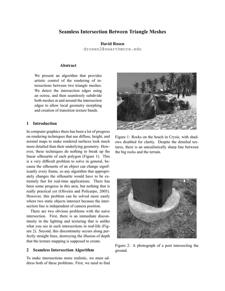
Seamless Intersection Between Triangle Meshes
David Rosen
drosen2@swarthmore.edu
Abstract
We present an algorithm that provides
artistic control of the rendering of intersections between two triangle meshes.
We detect the intersection edges using
an octree, and then seamlessly subdivide
both meshes at and around the intersection
edges to allow local geometry morphing
and creation of transition texture bands.
1
Introduction
In computer graphics there has been a lot of progress
on rendering techniques that use diffuse, height, and
normal maps to make rendered surfaces look much
more detailed than their underlying geometry. However, these techniques do nothing to break up the
linear silhouette of each polygon (Figure 1). This
is a very difficult problem to solve in general, because the silhouette of an object can change significantly every frame, so any algorithm that appropriately changes the silhouette would have to be extremely fast for real-time applications. There has
been some progress in this area, but nothing that is
really practical yet (Oliveira and Policarpo, 2005).
However, this problem can be solved more easily
where two static objects intersect because the intersection line is independent of camera position.
There are two obvious problems with the naive
intersection. First, there is an immediate discontinuity in the lighting and texturing that is unlike
what you see in such intersections in real-life (Figure 2). Second, this discontinuity occurs along perfectly straight lines, destroying the illusion of depth
that the texture mapping is supposed to create.
2
Seamless Intersection Algorithm
To make intersections more realistic, we must address both of these problems. First, we need to find
Figure 1: Rocks on the beach in Crysis, with shadows disabled for clarity. Despite the detailed textures, there is an unrealistically sharp line between
the big rocks and the terrain.
Figure 2: A photograph of a post intersecting the
ground.
the intersection between the objects and create vertices at each point of intersection. We can then find
auxiliary intersections which we will discuss auxiliary intersections in more detail in section 2.2, and
explain more clearly why they are important. Using
our new intersection and auxiliary intersection vertices, we can apply geometric deformations around
the intersections, and create texture bands to make
them look more natural. None of these steps are trivial, so we will explore them one at a time.
2.1 Data Structures
First, we should look at the data structures we are
using to represent the mesh. The mesh object contains an array of vertices and an array of triangles.
Each vertex object contains several vectors: a 3-part
vector storing its local coordinates, a 3-part vector
storing its surface normal, and a 2-part vector storing
its texture coordinates. Each triangle object contains
three pointers, one to each of its vertices.
2.2 Finding Intersection Segments
To find the intersection of two meshes, we could
check every triangle against every other triangle to
see if there is an intersection. However, this would
require O(n2 ) comparisons, which is not acceptable
when working with detailed meshes. Fortunately,
we can do much better using what I call an intersection octree (Figure 3), which indexes pairs of triangles that might intersect. Each node in the octree
contains the coordinates of its bounding box and two
lists of triangles (one for each mesh). We create the
root of the octree by taking the intersection of the
bounding boxes of each mesh, and adding all of the
triangles from each mesh that at least partially lie
within this shared bounding box. We then recursively subdivide each node until it reaches a maximum depth or no longer contains at least one triangle from each mesh. Finally, we walk through all of
the child nodes and report each pair of triangles, and
check each pair for intersection using well-known
techniques (Moller, 1997), returning the intersection
as a line segment. We have now efficiently found the
intersection between two meshes as a set of line segments (Figure 4), which will form a closed loop if
both meshes are closed.
Figure 3: The intersection octree generated by a
power transformer and a detailed sidewalk. The octree returned 70 pairs of triangles that might intersect, out of 846,000 possible pairs.
Figure 4: The intersection segments between a
power transformer and a sidewalk.
Figure 6: Scaling a model by moving vertices along
their normals, resulting in discontinuities at sharp
edges.
2.3 Finding Auxiliary Intersections
Figure 5: Without an auxiliary intersection (left),
the deformation propagates in an uncontrolled way.
With the auxiliary intersection (right), we have precise control over the shape of the deformation.
If we would like to change the geometry around
the intersecting object, we will need to find auxiliary intersections to protect the environment geometry from these changes(Figure 5). For example, if
a tree is intersecting the ground on a large, flat field
represented by a single triangle, then altering the intersection points will alter the geometry of the entire field. If we want to create a small slope in the
ground around the tree of some controlled size, say
two inches, then we can find the auxiliary points
by translating each vertex in the object out by two
inches in the direction of the surface normal. However, for meshes with sharp edges, the surface normals of overlapping vertices can point in different
directions, and moving each vertex along its surface
normal could result in a discontinuous mesh (Figure 6). We can solve this by temporarily averaging
together all normals belonging to overlapping vertices (Figure 7).
This can be done in O(n log n) time using a kdtree (Bentley, 1975). We loop through each vertex
in the model, and check if the tree is storing a vertex that has the same coordinates. If not, we add
the vertex to the tree. If so, we store a pointer to
the vertex that is already in the tree. Now for each
group of overlapping vertices, we have a representative vertex in the tree, and every other overlapping
vertex has a pointer to its representative. We find
the average normal for each representative vertex by
looping through the vertices again, adding each vertex’s normal to its representative’s normal, and then
normalizing it by dividing it by its length. Finally,
we can translate each vertex by some multiple of the
normal of its representative vertex.
Figure 8 is an example of typical auxiliary intersections that we can use to isolate the effects of manipulation of intersection points. These will also be
useful later to isolate texture transition effects, so we
do not have to apply them to any unnecessarily large
triangles (so we can avoid drawing too many unnecessary pixels). It is essential to find and store all
of the lines of intersection, including auxiliary intersection, before the final retriangulation. Otherwise
we will have to find intersections with the triangles
that are already subdivided, and the algorithm will
take longer and end up with many unnecessary subdivisions.
2.4 Dividing Polygons Along Intersection Lines
Figure 7: Scaling a model by moving vertices along
their corrected normals. This results in some distortion, but no discontinuities
Now that we have our intersection segments, what
do we do with them? We have to retriangulate our
mesh to include these segments as edges, and we
have to do it without any cosmetic changes. That
is, the retriangulation itself should have no visible
effect on the scene, but we can use our new vertices later to change the intersection however we
like. This problem can be divided further into two
subproblems: creating the new vertices, and retriangulating the mesh to include the new edges.
2.4.1 Seamlessly Adding Vertices
Suppose we have an intersection point on the edge
of a triangle. How do we incorporate it into the
mesh? We know the position component already,
but our mesh vertices contain other auxiliary information, such as texture coordinates and surface normals. Since our vertex is on an edge, we can just
Figure 9: The Delaunay triangulation (right) does
not necessarily preserve the lines of intersection
(left).
Figure 8: Some examples of auxiliary intersections
Figure 10: The constrained Delaunay triangulation
(right) is guaranteed to preserve the lines of intersection (left).
2.4.2 Retriangulation
interpolate between the auxiliary information stored
in the two endpoint vertices based on their relative
distance from the new point. But what if our intersection point is not on an edge? Suddenly the problem is much more complicated. We still have to interpolate between the three vertices, but it is not as
obvious what weights to assign to each vertex in the
interpolation.
The solution here is to find the position of the intersection point in barycentric coordinates. That is,
find its position as a weighted sum of the positions of
the three triangle vertices. So far this sounds somewhat circular: how do we find the barycentric coordinates? We know that the weighted sum of the
triangle vertices in each axis adds up to our new vertex, and we know that the weights have to add up to
1. We have a system of four independent equations
and three unknowns, so we can just solve it using
linear algebra. Once we have the weights of each
triangle vertex, we can use them to interpolate all of
the auxiliary values of our new vertex.
Now that we have our seamless vertices, how do
we incorporate them into the triangulation? At first
we expected that we could just use Delaunay triangulation on the set of intersection points and triangle vertices, but that failed because it did not preserve our lines of intersection (Figure 9). To achieve
the desired results, we had to use the constrained
Delaunay triangulation, which takes as input a set
of points as well as a set of line segments to preserve(Figure 10). Implementing the constrained
Delaunay triangulation efficiently could easily be a
final project in itself, so we used the free “Triangle”
library (Shewchuk, 2002).
2.5 Geometry Morphing
To deform the geometry, we can now safely translate
any of intersection vertices that do not lie on the outermost auxiliary intersection ring. After moving any
of the vertices, we have to recalculate the normals of
all of the adjacent triangles so that the lighting will
be correct for their new orientation. With one intersection ring and two auxiliary intersection rings,
Figure 11: Translating upwards the intersection ring
and inner auxiliary intersection ring.
Figure 12: Translating upwards only the inner auxiliary intersection ring.
we can create a number of interesting effects. We
can raise the intersection ring and the inner auxiliary ring to slope the ground around the object (Figure 11), or we can only raise the inner auxiliary ring
to create a crater effect (Figure 12).
2.6 Texture Band
Our final step is to create a texture band around the
intersection. First we will have to create a new mesh
that contains a copy of all the triangles and vertices
that we will need, and then we will have to assign
texture coordinates to each vertex in the mesh. To
create the new mesh, we can make a copy of each
triangle that contains at least one of the intersection
points, and make a copy of each of its vertices. If it
fits the effect we are going for, we can now recalcu-
late the normals to smooth the lighting transition at
the intersection. Alternately, we can leave them how
they are to keep the sharp edge.
Finally we have to calculate the texture coordinates. We would like to map the texture in Figure 13
to achieve the effect shown in Figure 14 and Figure
15. The vertical texture coordinate can be assigned
quite simply. Vertices on the intersection ring receive the vertical texture coordinate of 0.5, so that
it is lined up exactly with the center of the texture.
Vertices on the innermost auxiliary intersection ring
of one mesh receive the vertical texture coordinate
of 1.0, and of the other mesh, 0.0. This stretches the
texture over the intersection such that the middle of
the texture corresponds to the intersection ring, and
the top and bottom stretch out to the innermost auxiliary ring of each mesh.
The horizontal texture coordinates are a bit more
tricky. We have two priorities here: we would like
the texture to be mapped with uniform density, and
we would like it to wrap around seamlessly. Mapping it with uniform density means that it is never
stretched or compressed. That is, the difference in
texture coordinate between two connected vertices is
proportional to the physical distance between them.
To satisfy this constraint, we can start at any intersection point and assign it a horizontal texture coordinate of 0.0, and walk around the intersection, and
assign to each point a texture coordinate equal to the
total distance walked so far.
To satisfy the second constraint (seamless texture
wrapping), we have to round up to the nearest integer the total distance. That is, if the total distance
walked is 1.58 units, we have to round it to 2.0 units,
and scale all of the other texture coordinates similarly. We do this because the right edge of the texture
image lines up seamlessly with the left edge of the
texture image, and the only way that these can line
up on the texture band is if the image is repeated an
integral number of times. If the texture is repeated
1.58 times, then there will be a visible seam where
the texture coordinate wraps from 1.58 back to 0.0.
Now that we have the horizontal texture coordinates for the intersection points, we need horizontal
texture coordinates for the remaining points. To find
these we simply loop through all of the remaining
points and find the nearest intersection point, and
copy its horizontal texture coordinate. We can do
Figure 14: A subtle dirt texture (right) around the
base of an object.
Figure 13: A simple dirt texture that can be used for
texture bands.
this in O(n) time instead of O(n2 ) by only looking
at points that are connected by a triangle edge.
3
Results
This algorithm allows for artistic control of mesh
intersections, from subtle weathering effects (Figure 14) to dramatic impact deformations (Figure
12). It accomplishes this in O(n log n) time. In
this prototype implementation it takes about 0.2 seconds to create the intersections for the simple power
transformers ( 400 triangles), and about 1.6 seconds
to create the intersections for the detailed boulder
( 2500 triangles).
The intersection rings and retriangulation are robust to degenerate cases, but the deformation and
texture band creation can give unexpected results in
some cases. For example, the current deformation
algorithm will only affect vertices that are on one of
the intersection rings, so if there are other vertices
within the deformed area, there can be unexpected
indentations. Similarly, the texture bands stretch out
to the nearest vertices connected to the intersection
rings, which may not be the auxiliary intersection
rings if there are already vertices nearby.
Figure 15: A large dirt texture around the base of an
object.
4
Discussion and Future Work
There are many applications for this kind of technology. Two of the most significant applications are aging effects (e.g. rust accumulation around the base
of nails) or ambient occlusion (obstruction of ambient light when two surfaces are close together).
The algorithm takes a fraction of a second to run,
so with some optimization it will be useful for dynamic heightmaps, such as water surfaces, and dynamic environmental damage from explosions and
heavy impacts.
In the future we would like to make the deformation and texture bands more predictable in degenerate cases, and optimize the algorithm to run faster.
We would also like to create a user-friendly interface that allows artists to easily create and test new
kinds of intersection effects.
5
Conclusion
Intersections between detailed meshes have been a
serious problem in modern 3D graphics. We have
created an algorithm that can automatically create
deformations or texture bands that can greatly improve the appearance of these intersections. As far
as we know, there has been no other work addressing
this issue, so this is an important new step towards
efficiently creating realistic 3D environments.
References
Jon Louis Bentley. 1975. Multidimensional binary
search trees used for associative searching. Commun.
ACM, 18(9):509–517.
Tomas Moller. 1997. A fast triangle-triangle intersection
test. Journal of Graphics Tools, 2(2):25–30.
Manuel M. Oliveira and Fabio Policarpo. 2005. An efficient representation for surface details. UFRGS Technical Report, RP-351.
Jonathan Richard Shewchuk. 2002. Delaunay refinement algorithms for triangular mesh generation. Computational Geometry: Theory and Applications, 22(13):21–74.