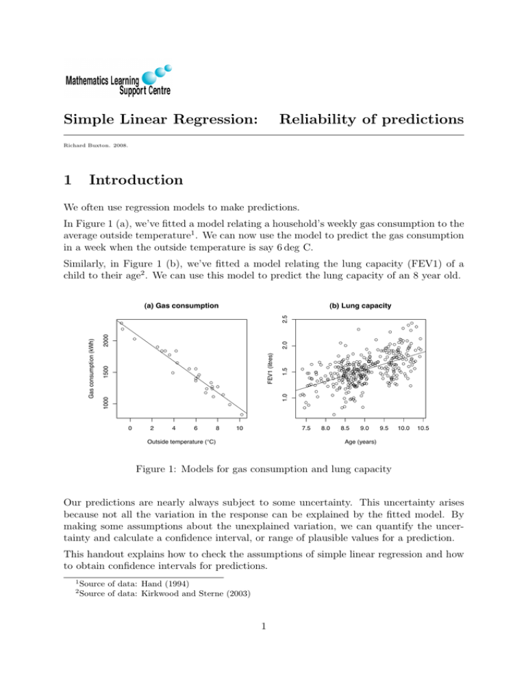
Simple Linear Regression:
Reliability of predictions
Richard Buxton. 2008.
1
Introduction
We often use regression models to make predictions.
In Figure 1 (a), we’ve fitted a model relating a household’s weekly gas consumption to the
average outside temperature1 . We can now use the model to predict the gas consumption
in a week when the outside temperature is say 6 deg C.
Similarly, in Figure 1 (b), we’ve fitted a model relating the lung capacity (FEV1) of a
child to their age2 . We can use this model to predict the lung capacity of an 8 year old.
(b) Lung capacity
1.0
1.5
FEV1 (litres)
2.0
2000
1500
1000
Gas consumption (kWh)
2.5
(a) Gas consumption
0
2
4
6
8
10
7.5
8.0
8.5
9.0
9.5
10.0
10.5
Age (years)
Outside temperature (°C)
Figure 1: Models for gas consumption and lung capacity
Our predictions are nearly always subject to some uncertainty. This uncertainty arises
because not all the variation in the response can be explained by the fitted model. By
making some assumptions about the unexplained variation, we can quantify the uncertainty and calculate a confidence interval, or range of plausible values for a prediction.
This handout explains how to check the assumptions of simple linear regression and how
to obtain confidence intervals for predictions.
1
2
Source of data: Hand (1994)
Source of data: Kirkwood and Sterne (2003)
1
If you’re new to regression analysis, you’ll probably find it useful to read the leaflet ‘Simple
Linear Regression: Introduction’ before continuing with this one.
2
Assumptions of simple linear regression
We make the following assumptions. . .
• Mean response varies linearly with predictor
• Unexplained variation is Normally and independently distributed with constant variance
To check these assumptions, we look at plots of the residuals and fitted values. The fitted
values are the values of the response predicted by the model. The residuals are obtained
by taking the observed values of the response and subtracting the fitted values. The two
most useful plots are. . .
• Plot of Residuals vs Fitted values
10
0
Residuals
5
30
20
!5
10
0
Stopping distance (metres)
40
– We can use this plot to check the assumptions of linearity and constant variance. For example, Figure 2 shows some plots for a regression model relating
stopping distance to speed3 . The plot on the left shows the data, with a fitted
linear model. The plot on the right shows the residuals plotted against the
fitted values - a smooth curve has been added to highlight the pattern of the
plot.
5
10
15
20
25
30
35
40
0
Speed (mph)
5
10
20
Fitted values
Figure 2: Stopping distance vs Speed
3
15
Source of data: Hand (1994)
2
25
30
0.5
!0.5
0.0
Residuals
0.0
!0.5
Residuals
0.5
Ideally, the residual plot should show a horizontal band of roughly equal width.
In this case, we have a strong ‘U’ shape, suggesting that the residuals go from
positive to negative to positive. This suggests that we’re fitting a line to a
non-linear relationship - see plot of original data. In addition, the width of the
band of data increases from the left to the right, suggesting that the variance
is increasing. There are various courses of action that we can take to deal with
these problems - for details, consult a Statistician.
Figure 3 shows some diagnostic plots for the regression of lung capacity on
age that we looked at in Section 1. Looking at the plot of residuals vs fitted
values, we have a horizontal band of data of roughly constant width. So the
assumptions of linearity and constant variance do seem to hold here.
1.2
1.3
1.4
1.5
1.6
1.7
1.8
!3
Fitted values
!2
!1
0
1
2
3
Theoretical Quantiles
Figure 3: Diagnostic plots for Lung data
• Normal probability plot of residuals
– This plot is used to check the assumption that the unexplained variation follows a Normal distribution. Normality is indicated by a roughly linear plot.
Any strong systematic curvature suggests some degree of non-Normality. The
Normal plot in Figure 3 is roughly linear, confirming that the unexplained
variation is roughly Normal.
There are several ways of checking the assumption that the random variation is statistically independent. For details, see Koop (2008). The assumption of independence is not
usually a problem except for data that has been collected at successive points in time e.g. monthly unemployment figures.
3
3
Checking assumptions in SPSS
—Analyse
—Regression
—Linear
—drag the response variable into the Dependent box
—drag the predictor variable into the Independent(s) box
—Plots
—drag the residuals (*ZRESID) into the Y box
—drag the fitted values (*ZPRED) into the X box
—Select Normal Probability Plot
—Click Continue
—Click OK
Use the plot of Residuals against Fitted values to check for any evidence of non-linearity
or non-constant variance. Use the Normal probability plot to check for evidence of nonNormality.
4
Confidence intervals for predictions
Provided the assumptions in Section 2 are satisfied, we can obtain confidence intervals
for any predictions that we make.
We illustrate with the example on lung capacity (FEV1) vs age. The fitted model is. . .
F = −0.475 + 0.224 A
. . . where F is FEV1 and A is Age.
Suppose we want to predict FEV1 for a child of 9. We can obtain a point prediction
by simply substituting 9 in place of A in the fitted model. But calculating a confidence
interval is more difficult, so in practice, we use statistical software to make our predictions.
There are two types of confidence interval. . .
• Confidence interval for individual case
– Range of plausible values for a single case - e.g. for the FEV1 of a single child
• Confidence interval for mean
– Range of plausible values for the mean - e.g. for the mean FEV1 over a large
number of children, all of the same age.
4
Table 1 shows the SPSS output for age 9.
Age PRE 1 LMCI 1 UMCI 1 LICI 1 UICI 1
9.00 1.53695 1.51102 1.56288 1.06161 2.01229
Table 1: Prediction and confidence intervals
If we’re predicting the FEV1 for a single child, we use the columns headed LICI 1 (Lower
Individual Confidence Interval) and UICI 1 (Upper Individual Confidence Interval).
95% confidence interval
1.06 to 2.01 litres
We can be fairly sure that the FEV1 value will lie within this range.
If we wished to predict the mean value of FEV1 for a large group of children, all of age
9, we would use the columns LMCI 1 and UMCI 1.
95% confidence interval for mean
1.51 to 1.56 litres
This interval is much narrower. We’re much less sure about the lung function of a single
child than we are about the mean lung function for a large group of children.
5
Making predictions in SPSS
Go to the SPSS Data Editor and add the new predictor values (i.e. the values at which
you wish to make predictions) to the bottom of the column containing the predictor.
—Analyse
—Regression
—Linear
—drag the response variable into the Dependent box
—drag the predictor variable into the Independent(s) box
—Save
—under Predicted Values, select Unstandardized
—under Prediction Intervals, select Mean or Individual
—Click Continue
—Click OK
SPSS calculates the predicted values and confidence intervals and puts them in five new
columns in the Data Editor window.
5
6
Confidence interval for slope of regression model
We’re sometimes interested in the change in the response corresponding to a given change
in the predictor. For example, how much will our stopping distance increase if we travel
10mph faster? We can answer this kind of question by looking at the slope of the regression
line.
Table 2 shows some SPSS output giving the coefficients of the Lung model, together with
confidence intervals for both the slope and intercept.
Model
1
(Constant)
A
Coefficients
Unstandardized 95% Conf Int for B
Coefficients
Lower
Upper
B
Std.Error Bound
Bound
-.475
.164
-.798
-.153
.224
.018
.188
.259
Table 2: Confidence intervals for coefficients
The coefficient of A is 0.224. This tells us that an increase of one year in age is associated
with an increase in FEV1 of around 0.224 litres. The columns on the right of the table
give a confidence interval for this figure.
95% confidence interval
0.188 to 0.259 litres
This gives us a range of plausible values for the increase in FEV1 corresponding to a unit
increase in age.
If we’re interested in the change in FEV1 corresponding to say a two year increase in age,
we can obtain a confidence interval by simply multiplying the lower and upper ends of
our confidence interval by 2 to give. . .
95% confidence interval
7
0.376 to 0.518 litres.
Estimating the slope in SPSS
—Analyse
—Regression
—Linear
—drag the response variable into the Dependent box
—drag the predictor variable into the Independent(s) box
—Statistics
—under Regression Coefficient, select Confidence Intervals
—Click Continue
—Click OK
The table of coefficients will now include confidence intervals for the intercept and slope.
6
8
References
For a simple introduction to regression, see Moore and McCabe (2004). For a more
comprehensive treatment, see Freund and Wilson (1998).
Freund, R.J. and Wilson, W.J. (1998). Regression Analysis: statistical Modeling
of a Response Variable, Academic Press.
Hand, D.J. (1994). A Handbook of Small Data Sets, Chapman and Hall.
Kirkwood, B.R. and Sterne, J.A.C. (2003). Essential Medical Statistics, Blackell
Science.
Koop, G. (2008). Introduction to Econometrics, Wiley.
Moore, D.S. and McCabe, G.P. (2004). Introduction to the practice of statistics,
5th edition, W.H.Freeman.
7