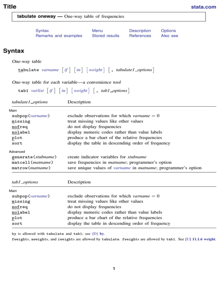
Title
stata.com
tabulate oneway — One-way table of frequencies
Syntax
Remarks and examples
Menu
Stored results
Description
References
Options
Also see
Syntax
One-way table
tabulate varname
if
in
weight
, tabulate1 options
One-way table for each variable—a convenience tool
tab1 varlist if
in
weight
, tab1 options
tabulate1 options
Description
Main
subpop(varname)
missing
nofreq
nolabel
plot
sort
exclude observations for which varname = 0
treat missing values like other values
do not display frequencies
display numeric codes rather than value labels
produce a bar chart of the relative frequencies
display the table in descending order of frequency
Advanced
generate(stubname)
matcell(matname)
matrow(matname)
create indicator variables for stubname
save frequencies in matname; programmer’s option
save unique values of varname in matname; programmer’s option
tab1 options
Description
Main
subpop(varname)
missing
nofreq
nolabel
plot
sort
exclude observations for which varname = 0
treat missing values like other values
do not display frequencies
display numeric codes rather than value labels
produce a bar chart of the relative frequencies
display the table in descending order of frequency
by is allowed with tabulate and tab1; see [D] by.
fweights, aweights, and iweights are allowed by tabulate. fweights are allowed by tab1. See [U] 11.1.6 weight.
1
2
tabulate oneway — One-way table of frequencies
Menu
tabulate oneway
Statistics
>
Summaries, tables, and tests
>
Frequency tables
>
One-way table
tabulate ..., generate()
Data
>
Create or change data
>
Other variable-creation commands
>
Create indicator variables
tab1
Statistics
>
Summaries, tables, and tests
>
Frequency tables
>
Multiple one-way tables
Description
tabulate produces a one-way table of frequency counts.
For information about a two-way table of frequency counts along with various measures of
association, including the common Pearson χ2 , the likelihood-ratio χ2 , Cramér’s V , Fisher’s exact
test, Goodman and Kruskal’s gamma, and Kendall’s τb , see [R] tabulate twoway.
tab1 produces a one-way tabulation for each variable specified in varlist.
Also see [R] table and [R] tabstat if you want one-, two-, or n-way table of frequencies and a wide
variety of summary statistics. See [R] tabulate, summarize() for a description of tabulate with the
summarize() option; it produces a table (breakdowns) of means and standard deviations. table is
better than tabulate, summarize(), but tabulate, summarize() is faster. See [ST] epitab for
a 2 × 2 table with statistics of interest to epidemiologists.
Options
Main
subpop(varname) excludes observations for which varname = 0 in tabulating frequencies. The
mathematical results of tabulate . . ., subpop(myvar) are the same as tabulate . . . if myvar
!=0, but the table may be presented differently. The identities of the rows and columns will be
determined from all the data, including the myvar = 0 group, so there may be entries in the table
with frequency 0.
Consider tabulating answer, a variable that takes on values 1, 2, and 3, but consider tabulating
it just for the male==1 subpopulation. Assume that answer is never 2 in this group. tabulate
answer if male==1 produces a table with two rows: one for answer 1 and one for answer 3.
There will be no row for answer 2 because answer 2 was never observed. tabulate answer,
subpop(male) produces a table with three rows. The row for answer 2 will be shown as having
0 frequency.
missing requests that missing values be treated like other values in calculations of counts, percentages,
and other statistics.
nofreq suppresses the printing of the frequencies.
nolabel causes the numeric codes to be displayed rather than the value labels.
plot produces a bar chart of the relative frequencies in a one-way table. (Also see [R] histogram.)
sort puts the table in descending order of frequency (and ascending order of the variable within
equal values of frequency).
tabulate oneway — One-way table of frequencies
3
Advanced
generate(stubname) creates a set of indicator variables (stubname1, stubname2, . . . ) reflecting the
observed values of the tabulated variable. The generate() option may not be used with the by
prefix.
matcell(matname) saves the reported frequencies in matname. This option is for use by programmers.
matrow(matname) saves the numeric values of the r × 1 row stub in matname. This option is for
use by programmers. matrow() may not be specified if the row variable is a string.
Limits
A one-way table may have a maximum of 12,000 rows (Stata/MP and Stata/SE), 3,000 rows
(Stata/IC), or 500 rows (Small Stata).
Remarks and examples
stata.com
Remarks are presented under the following headings:
tabulate
tab1
Video example
For each value of a specified variable, tabulate reports the number of observations with that
value. The number of times a value occurs is called its frequency.
tabulate
Example 1
We have data summarizing the speed limit and the accident rate per million vehicle miles along
various Minnesota highways in 1973. The variable containing the speed limit is called spdlimit. If
we summarize the variable, we obtain its mean and standard deviation:
. use http://www.stata-press.com/data/r13/hiway
(Minnesota Highway Data, 1973)
. summarize spdlimit
Variable
Obs
Mean
spdlimit
39
55
Std. Dev.
Min
Max
5.848977
40
70
The average speed limit is 55 miles per hour. We can learn more about this variable by tabulating it:
. tabulate spdlimit
Speed Limit
Freq.
Percent
Cum.
40
45
50
55
60
65
70
1
3
7
15
11
1
1
2.56
7.69
17.95
38.46
28.21
2.56
2.56
2.56
10.26
28.21
66.67
94.87
97.44
100.00
Total
39
100.00
4
tabulate oneway — One-way table of frequencies
We see that one highway has a speed limit of 40 miles per hour, three have speed limits of 45, 7
of 50, and so on. The column labeled Percent shows the percentage of highways in the dataset
that have the indicated speed limit. For instance, 38.46% of highways in our dataset have a speed
limit of 55 miles per hour. The final column shows the cumulative percentage. We see that 66.67%
of highways in our dataset have a speed limit of 55 miles per hour or less.
Example 2
The plot option places a sideways histogram alongside the table:
. tabulate spdlimit, plot
Speed Limit
Freq.
40
45
50
55
60
65
70
1
3
7
15
11
1
1
Total
39
*
***
*******
***************
***********
*
*
Of course, graph can produce better-looking histograms; see [R] histogram.
Example 3
tabulate labels tables using variable and value labels if they exist. To demonstrate how this
works, let’s add a new variable to our dataset that categorizes spdlimit into three categories. We
will call this new variable spdcat:
. generate spdcat=recode(spdlimit,50,60,70)
The recode() function divides spdlimit into 50 miles per hour or below, 51 – 60, and above 60;
see [D] functions. We specified the breakpoints in the arguments (spdlimit,50,60,70). The first
argument is the variable to be recoded. The second argument is the first breakpoint, the third argument
is the second breakpoint, and so on. We can specify as many breakpoints as we wish.
recode() used our arguments not only as the breakpoints but also to label the results. If spdlimit
is less than or equal to 50, spdcat is set to 50; if spdlimit is between 51 and 60, spdcat is 60;
otherwise, spdcat is arbitrarily set to 70. (See [U] 25 Working with categorical data and factor
variables.)
Because we just created the variable spdcat, it is not yet labeled. When we make a table using
this variable, tabulate uses the variable’s name to label it:
. tabulate spdcat
spdcat
Freq.
Percent
Cum.
50
60
70
11
26
2
28.21
66.67
5.13
28.21
94.87
100.00
Total
39
100.00
tabulate oneway — One-way table of frequencies
5
Even through the table is not well labeled, recode()’s coding scheme provides us with clues as to
the table’s meaning. The first line of the table corresponds to 50 miles per hour and below, the next
to 51 through 60 miles per hour, and the last to above 60 miles per hour.
We can improve this table by labeling the values and variables:
. label define scat 50 "40 to 50" 60 "55 to 60" 70 "Above 60"
. label values spdcat scat
. label variable spdcat "Speed Limit Category"
We define a value label called scat that attaches labels to the numbers 50, 60, and 70 using the
label define command; see [U] 12.6.3 Value labels. We label the value 50 as ‘40 to 50’, because
we looked back at our original tabulation in the first example and saw that the speed limit was never
less than 40. Similarly, we could have labeled the last category ‘65 to 70’ because the speed limit
is never greater than 70 miles per hour.
Next we requested that Stata label the values of the new variable spdcat using the value label
scat. Finally, we labeled our variable Speed Limit Category. We are now ready to tabulate the
result:
. tabulate spdcat
Speed Limit
Category
Freq.
Percent
Cum.
40 to 50
55 to 60
Above 60
11
26
2
28.21
66.67
5.13
28.21
94.87
100.00
Total
39
100.00
Example 4
If we have missing values in our dataset, tabulate ignores them unless we explicitly indicate
otherwise. We have no missing data in our example, so let’s add some:
. replace spdcat=. in 39
(1 real change made, 1 to missing)
We changed the first observation on spdcat to missing. Let’s now tabulate the result:
. tabulate spdcat
Speed Limit
Category
Freq.
Percent
Cum.
40 to 50
55 to 60
Above 60
11
26
1
28.95
68.42
2.63
28.95
97.37
100.00
Total
38
100.00
Comparing this output with that in the previous example, we see that the total frequency count is now
one less than it was — 38 rather than 39. Also, the ‘Above 60’ category now has only one observation
where it used to have two, so we evidently changed a road with a high speed limit.
We want tabulate to treat missing values just as it treats numbers, so we specify the missing
option:
6
tabulate oneway — One-way table of frequencies
. tabulate spdcat, missing
Speed Limit
Category
Freq.
Percent
Cum.
28.21
94.87
97.44
100.00
40 to 50
55 to 60
Above 60
.
11
26
1
1
28.21
66.67
2.56
2.56
Total
39
100.00
We now see our missing value — the last category, labeled ‘.’, shows a frequency count of 1. The
table sum is once again 39.
Let’s put our dataset back as it was originally:
. replace spdcat=70 in 39
(1 real change made)
Technical note
tabulate also can automatically create indicator variables from categorical variables. We will
briefly review that capability here, but see [U] 25 Working with categorical data and factor variables
for a complete description. Let’s begin by describing our highway dataset:
. describe
Contains data from http://www.stata-press.com/data/r13/hiway.dta
obs:
39
Minnesota Highway Data, 1973
vars:
3
16 Nov 2012 12:39
size:
351
variable name
storage
type
display
format
value
label
spdlimit
rate
byte
float
%8.0g
%9.0g
rcat
spdcat
float
%9.0g
scat
Sorted by:
Note:
variable label
Speed Limit
Accident rate per million vehicle
miles
Speed Limit Category
dataset has changed since last saved
Our dataset contains three variables. We will type tabulate spdcat, generate(spd), describe
our data, and then explain what happened.
. tabulate spdcat, generate(spd)
Speed Limit
Category
Freq.
Percent
40 to 50
55 to 60
Above 60
11
26
2
28.21
66.67
5.13
Total
39
100.00
Cum.
28.21
94.87
100.00
tabulate oneway — One-way table of frequencies
7
. describe
Contains data from http://www.stata-press.com/data/r13/hiway.dta
obs:
39
Minnesota Highway Data, 1973
vars:
6
16 Nov 2012 12:39
size:
468
variable name
storage
type
display
format
value
label
rcat
spdlimit
rate
byte
float
%8.0g
%9.0g
spdcat
spd1
spd2
spd3
float
byte
byte
byte
%9.0g
%8.0g
%8.0g
%8.0g
Sorted by:
Note:
scat
variable label
Speed Limit
Accident rate per million vehicle
miles
Speed Limit Category
spdcat==40 to 50
spdcat==55 to 60
spdcat==Above 60
dataset has changed since last saved
When we typed tabulate with the generate() option, Stata responded by producing a one-way
frequency table, so it appeared that the option did nothing. Yet when we describe our dataset, we
find that we now have six variables instead of the original three. The new variables are named spd1,
spd2, and spd3.
When we specify the generate() option, we are telling Stata to not only produce the table but
also create a set of indicator variables that correspond to that table. Stata adds a numeric suffix to
the name we specify in the parentheses. spd1 refers to the first line of the table, spd2 to the second
line, and so on. Also Stata labels the variables so that we know what they mean. spd1 is an indicator
variable that is true (takes on the value 1) when spdcat is between 40 and 50; otherwise, it is zero.
(There is an exception: if spdcat is missing, so are the spd1, spd2, and spd3 variables. This did
not happen in our dataset.)
We want to prove our claim. Because we have not yet introduced two-way tabulations, we will
use the summarize statement:
. summarize spdlimit if spd1==1
Obs
Mean
Variable
spdlimit
11
47.72727
. summarize spdlimit if spd2==1
Obs
Mean
Variable
spdlimit
26
57.11538
. summarize spdlimit if spd3==1
Variable
Obs
Mean
spdlimit
2
67.5
Std. Dev.
Min
Max
3.437758
40
50
Std. Dev.
Min
Max
2.519157
55
60
Std. Dev.
Min
Max
3.535534
65
70
Notice the indicated minimum and maximum in each of the tables above. When we restrict the
sample to spd1, spdlimit is between 40 and 50; when we restrict the sample to spd2, spdlimit
is between 55 and 60; when we restrict the sample to spd3, spdlimit is between 65 and 70.
Thus tabulate provides an easy way to create indicator (sometimes called dummy) variables.
For an overview of indicator and categorical variables, see [U] 25 Working with categorical data
and factor variables.
8
tabulate oneway — One-way table of frequencies
tab1
tab1 is a convenience tool. Typing
. tab1 myvar thisvar thatvar, plot
is equivalent to typing
. tabulate myvar, plot
. tabulate thisvar, plot
. tabulate thatvar, plot
Video example
Tables and cross-tabulations in Stata
Stored results
tabulate and tab1 store the following in r():
Scalars
r(N)
number of observations
r(r)
number of rows
References
Cox, N. J. 2009. Speaking Stata: I. J. Good and quasi-Bayes smoothing of categorical frequencies. Stata Journal 9:
306–314.
Harrison, D. A. 2006. Stata tip 34: Tabulation by listing. Stata Journal 6: 425–427.
Also see
[R] table — Flexible table of summary statistics
[R] tabstat — Compact table of summary statistics
[R] tabulate twoway — Two-way table of frequencies
[R] tabulate, summarize() — One- and two-way tables of summary statistics
[D] collapse — Make dataset of summary statistics
[ST] epitab — Tables for epidemiologists
[SVY] svy: tabulate oneway — One-way tables for survey data
[SVY] svy: tabulate twoway — Two-way tables for survey data
[XT] xttab — Tabulate xt data
[U] 12.6.3 Value labels
[U] 25 Working with categorical data and factor variables