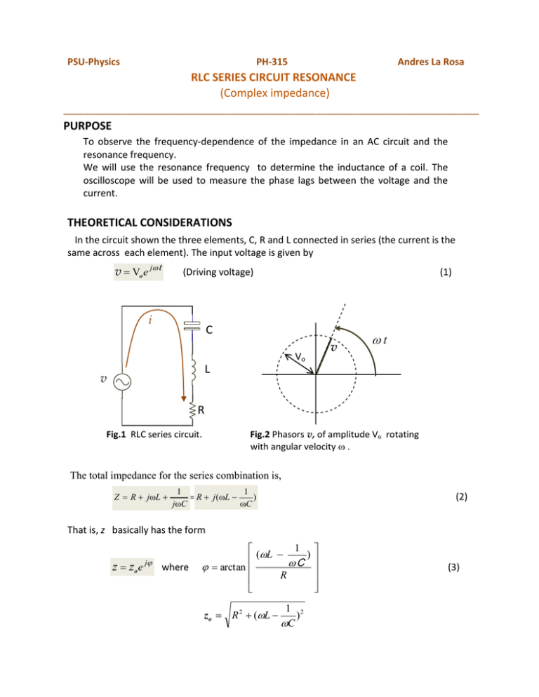
PSU-Physics
PH-315
Andres La Rosa
RLC SERIES CIRCUIT RESONANCE
(Complex impedance)
_______________________________________________________________________________
PURPOSE
To observe the frequency-dependence of the impedance in an AC circuit and the
resonance frequency.
We will use the resonance frequency to determine the inductance of a coil. The
oscilloscope will be used to measure the phase lags between the voltage and the
current.
THEORETICAL CONSIDERATIONS
In the circuit shown the three elements, C, R and L connected in series (the current is the
same across each element). The input voltage is given by
v  Vo e j t
(Driving voltage)
i
(1)
C
v
Vo
t
L
v
R
Fig.1 RLC series circuit.
Fig.2 Phasors v, of amplitude Vo rotating
with angular velocity 
The total impedance for the series combination is,
Z  R  jL 
1
1
)
= R  j (L 
jC
C
(2)
That is, z basically has the form
z  zo e
j
where
1

 (L   C )
  arctan 
R


zo  R 2  (L 
1 2
)
C





(3)

L

R
L – 1/(C)
1/(C)
Fig.3 Representation of the impedance in the complex plane.
From (1) and (2), one obtain the current,
i
v
1

v
Z R  j (L  1 )
C
(4)
Or, equivalently,
i
i
1
e -j
v

v 
zo
zo e j
1
1 2
R  (L 
)
C
e -j
1 2
R  (L 
)
C
v
2
e  j v
(5)
2

This result indicates the following:


v
i
se is measured relative to
v
i
Case: > 0
Case: < 0
Fig.4 Phases voltage and current rotating counterclockwise. Left:
The current lags the voltage. Right: The current leads the voltage.
Using (1) in (5),
i
Vo
1 2
R  (L 
)
C
2
e j(  t -  ) 
Ie
j ( t -  )
(6)
1

 (L   C )
  arctan 
R


where





Notice,
  -  (current leads the voltage)
at very low frequencies:
at   o 
1
we have:=
LC
at very high frequencies


v
   (current lags the voltage)
i

v

v
i
v
i

~ 0
~ 0
Fig.5 Change of phase as the frequency varies
Notice in (3) and (6) that when L  1 /(C) ,
The impedance is minimum
The current is maximum
Hence   o 
i
1
is called the resonance frequency.
LC


Fig.6 Resonance curve

  ∞

EXPERIMENTAL CONSIDERATIONS
The oscilloscope is our basic measuring tool in alternating current (AC) circuits.
The resistor Ro is a known resistor (whose value is on the order of 100 ). The ground of the
oscilloscope will be connected to G, while the two inputs will be to points A and B.
GA will measure the input voltage VA , while
GB will measure VR = IR0 from which the current I can be deduced.
Measure the frequency of the input voltage using the oscilloscope. (Do not trust the reading from
the signal generator knob).
Note: In atypical capacitor, labeled, for example 473G, it means C = 47x10 3 picoFarads.
(Suggestion: use C~ 10 nF for this experiment.)
MEASUREMENTS
a) The magnitude of the impedance Z of the test circuit is determined from the ratio of
amplitudes of the two signals, VA and I.
Plot |Z | as a function
of .
C= 10 nF
b) The phase can be measured on the
oscilloscope as a distance between the
points where the two traces cross the
horizontal axis, and converted to degrees
by comparing the half (or full) wavelength
as shown on the oscilloscope. See figure
below.
Pay attention during the measurements to
verify if  is positive or negative. That is,
whether the VR is lagging or ahead of VA.
A
L
B
Ground
Ro
G
Plot  = ()
Real voltages
Measured by the oscilloscope
Complex analysis
Phasors
VA
vA
t
 v
R
vR
time

180o
VA =Vo Cos (t); VR = Vo Cos (t - )
Phasors vA and vR rotating with
The traces show VR lagging VA by .
angular velocity vR lags vA by .
c) During the course of measurements you should take enough data to make a graph of both
impedance and phase as a function of frequency. How does the curve changes when using a
higher value of the resistance Ro?
In order to compare this to theory, you will need to determine tire value of the inductance L.
This is best done early in the exercise by locating the resonance frequency, where the
impedance is minimum and where the phase between VA and VR is zero. This is obviously the
frequency region where a majority of your data needs to be taken. The quality of your plot of
impedance and phase is more dependent upon taking data that spans the region of interest
than it is on the volume of data alone.
By rearranging the circuit elements and shifting the ground it is possible to compare the signals
across C and R, and across L and R.
d) At resonance condition, measure the voltage across the three elements (you will need to
swap C and L, one at a time, with the element R). Do these values add up?
e) Choose a frequency at which I is ~50% of Iresonance. Verify experimentally and corroborate
theoretically the validity of Kirchhoff law (measure the complex values for Vc, VL, VR?
OVERCOMING the SHORTCOMINGS ENCOUNTERED in the EXPERIMENT
Problem: Variability of the input voltage amplitude
Correction: By the normalization method.
While sweeping the frequency of the input voltage VA around the resonance frequency, it is
observed that the amplitude of the driving voltage also changes. Ideally, it would be desirable
that this amplitude remains constant.
The instability of the VA ‘s amplitude makes somewhat inaccurate the procedure of locating the
resonance frequency by monitoring the frequency at which the current is maximum. (When you
do this, you may find that at the frequency where the current is maximum, VA and I are not in
phase.) Still this is still a good preliminary step, since it helps to identify the frequency range
where we have to take a closer look.
Next, sweep the frequency a bit, until you find that the phase between VA and I is zero.
The suggested following step is to manually normalize the input voltage VA. By this we mean to
choose a fixed amplitude value for VA, let’s call it VA, fixed.
For a given frequency, record the current amplitude and phase.
Move to another frequency (you may notice that the amplitude of VA has changed.) Turn the
knob that controls the amplitude of VA until you obtain back the predetermined fixed value
VA, fixed. Then record the current amplitude and phase.
And so on, repeat the procedure for each frequency around the resonance frequency.
Or, i 
v
1

v , which gives,
Z R  j (L  1 )
C
1
i
R 2  (L 
1 2
)
C
e j v
where
1

 (L   C )
  arctan 
R







Notice,
at very low frequencies:
at   o 
1
we have:
LC
at very high frequencies
Thus we have,
= 

 - 
v  Vo e jt
iIe
i
 + 
j (t  )
(driving voltage)
 I e jt e j
(current)
dq
I j (t  )
I j (t  ) I j (t   / 2)
j (t   / 2)
implies q 
e
j e
 e
Qe
dt
j


q  Q e j (t   / 2)  Q e j (t  )Q e-j / 2
(charge)
q lags the current i by /2
k
Using the phasors representation,
A
Im
z  Ae
jt
x
z
m
t
Real
Real
Im
v
v
v
q
Real
q
q
At ~ 0
At ~ 0
At   ∞
Real
Im
i
v
Real
v
i
v
i
At ~ 0
At ~ 0
At   ∞