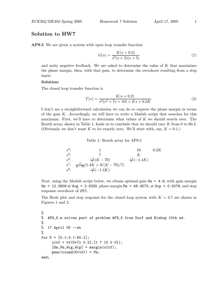
ECE382/ME482 Spring 2005
Homework 7 Solution
April 17, 2005
1
Solution to HW7
AP9.5 We are given a system with open loop transfer function
G(s) =
K(s + 0.2)
s2 (s + 2)(s + 5)
(1)
and unity negative feedback. We are asked to determine the value of K that maximizes
the phase margin, then, with that gain, to determine the overshoot resulting from a step
input.
Solution:
The closed loop transfer function is
T (s) =
K(s + 0.2)
.
s2 (s2 + 7s + 10) + Ks + 0.2K
(2)
I don’t see a straightforward calculation we can do to express the phase margin in terms
of the gain K. Accordingly, we will have to write a Matlab script that searches for this
maximum. First, we’ll have to determine what values of K we should search over. The
Routh array, shown in Table 1, leads us to conclude that we should vary K from 0 to 60.2.
(Obviously we don’t want K to be exactly zero. We’ll start with, say, K = 0.1.)
Table 1: Routh array for AP9.5
s4 :
s3 :
s2 :
s1 :
s0 :
1
7
−1
(K
− 70)
7
7
K−70 (1.4K + K(K − 70)/7)
−1
7 (−1.4K)
10
K
−1
(−1.4K)
7
0.2K
Next, using the Matlab script below, we obtain optimal gain Km = 4.9, with gain margin
Gm = 12.2809 at Wcg = 2.9320, phase margin Pm = 48.4573, at Wcp = 0.5078, and step
response overshoot of 29%.
The Bode plot and step response for the closed loop system with K = 3.7 are shown in
Figures 1 and 2.
%
% AP9_5.m solves part of problem AP9_5 from Dorf and Bishop 10th ed.
%
% 17 April 05 --sk
%
for K = [0.1:0.1:60.1];
oltf = tf(K*[1 0.2],[1 7 10 0 0]);
[Gm,Pm,Wcg,Wcp] = margin(oltf);
pmar(round(K*10)) = Pm;
end;
ECE382/ME482 Spring 2005
Homework 7 Solution
April 17, 2005
2
Figure 1: Closed Loop Bode Diagram for AP9.5 with K = 3.7
Closed Loop Bode Plot for AP9.5 with K = 4.9
50
Magnitude (dB)
0
−50
−100
−150
0
Phase (deg)
−90
−180
−270
−2
10
−1
10
0
10
Frequency (rad/sec)
1
10
[pmm,loc]=max(pmar);
Km = loc/10
oltf = tf(Km*[1 0.2],[1 7 10 0 0]);
cltf = feedback(oltf,1);
figure(5)
bode(cltf)
grid
title([’Closed Loop Bode Plot for AP9.5 with K = ’,num2str(Km)])
print -deps ap9_5a
[Gm,Pm,Wcg,Wcp] = margin(oltf)
[y,t] = step(cltf);
figure(6)
plot(t,y)
grid
% open loop not closed loop xfer fn!
2
10
ECE382/ME482 Spring 2005
Homework 7 Solution
April 17, 2005
3
Figure 2: Step Response for AP9.5 with K = 3.7
Step Response for AP9.5 with K = 4.9
1.4
1.2
1
y(t)
0.8
0.6
0.4
0.2
0
0
2
4
6
8
10
12
14
16
18
Time (s)
xlabel(’Time (s)’)
ylabel(’y(t)’)
title([’Step Response for AP9.5 with K = ’,num2str(Km)])
print -deps ap9_5aa
overshoot = max(y)
AP9.7 We are given a unity negative feedback system with compensator transfer function
K(s + 4) and plant transfer function 1/s2 cascaded in the forward path. A disturbance
input occurs between the compensator and the plant. We are asked to find a K that
results in phase margin of 45 degrees, then find the bandwidth and peak amplitude Mp
(not Mpω ) of the response to a unit step disturbance.
Solution: The closed loop transfer function is
T (s) =
K(s + 4)
Y (s)
= 2
R(s)
s + Ks + 4K
(3)
ECE382/ME482 Spring 2005
Homework 7 Solution
April 17, 2005
4
√
so the natural
frequency of the closed-loop system is ωn = 2 K and the damping coefficient
√
is ζ = K/4.
We’ll use an iterative search similar to that used in AP9.5, except that rather than maximizing the phase margin, we want to minimize the difference between the phase margin
and the design specified phase margin of 45 degrees. This time it is √
not so easy to determine the range of K to use. The poles of the system are −K/2 ± K 2 − 16K/2, so,
assuming that K is positive, the only way for a pole to have a positive real part is for the
square root to be real and greater than K. But, when real, the square root of K 2 − 16K
is always less than K. In other words, the gain does not affect the stability. That doesn’t
help us decide what range of K to check. Let’s start with the range 0 < K < 10 and, if
necessary, we’ll increase the upper bound.
Using the Matlab script below, we obtain optimal gain Km = 2.8, with infinite gain margin
and phase margin Pm = 44.8097, at Wcp = 3.9735. Using the interactive feature of the
Matlab Bode plot we determine that the system bandwidth is approximately 5.8 rad/s.
The maximum value of the closed loop step disturbance response is 2.8284.
The Bode plot and step response for the closed loop system with K = 2.8 are shown in
Figures 3 and 4.
%
% AP9_7.m solves part of problem AP9_7 from Dorf and Bishop 10th ed.
%
% 17 April 05 --sk
%
% iterate for closed loop gain margin
for K = [0.1:0.1:10];
oltf = tf(K*[1 4],[1 0 0]);
[Gm,Pm,Wcg,Wcp] = margin(oltf);
pmar(round(K*10)) = Pm;
end;
[foo,loc]=min(abs(pmar-45*ones(size(pmar))));
Km = loc/10
oltf = tf(Km*[1 4],[1 0 0]);
cltf = feedback(oltf,1);
figure(7)
bode(cltf)
grid
title([’Closed Loop Bode Plot for AP9.7 with K = ’,num2str(Km)])
print -deps ap9_7a
[Gm,Pm,Wcg,Wcp] = margin(oltf)
dcltf = tf(1,[1 Km 4*Km])
[y,t] = step(cltf);
figure(8)
ECE382/ME482 Spring 2005
Homework 7 Solution
April 17, 2005
5
Figure 3: Closed Loop Bode Diagram for AP9.7 with K = 2.8
Closed Loop Bode Plot for AP9.7 with K = 2.8
10
5
0
Magnitude (dB)
−5
−10
−15
−20
−25
−30
−35
−40
0
Phase (deg)
−45
−90
−135
−1
10
0
1
10
10
2
10
Frequency (rad/sec)
plot(t,y)
grid
xlabel(’Time (s)’)
ylabel(’y(t)’)
title([’Closed Loop Response to unit step disturbance for AP9.7 ’,...
’with K = ’,num2str(Km)])
print -deps ap9_7aa
max(y)
AP9.9 We are given a system with unity negative feedback and forward path transfer function
Gc (s)G(s) =
KP s + KI
s2 (s2 + 7s + 10)
(4)
where KI /KP = 0.2 and we are asked to find the value of KP that maximizes the phase
margin.
ECE382/ME482 Spring 2005
Homework 7 Solution
April 17, 2005
6
Figure 4: Closed Loop Step Disturbance Response for AP9.7 with K = 2.8
Closed Loop Response to unit step disturbance for AP9.7 with K = 2.8
1.4
1.2
1
y(t)
0.8
0.6
0.4
0.2
0
0
0.5
1
1.5
2
Time (s)
2.5
3
3.5
4
Solution: With KI /KP = 0.2, the closed loop transfer function is
T (s) =
s4
+
7s3
KP (s + 0.2)
.
+ 10s2 + KP (s + 0.2)
(5)
Conveniently, this is the same transfer function that we had in problem AP9.5. The
answer will thus be the same, i.e. Kp = 4.9 will yield the maximum phase margin, etc.
(Ok, so I wasn’t paying enough attention when I assigned this one. I trust there will be
no complaints. :-)
DP9.3 We are given a system having unity negative feedback and transfer function
G(s) =
Ke−10s
40s + 1
(6)
in the forward path. We are asked to choose a value for K to keep the output within a
narrow range while maintaining good dynamic response.
Solution: First, let’s generate a Bode diagram for the open loop system. The delay will
add φ(ω) = −ωT where T = 10 to the phase shift while not affecting the magnitude. We
ECE382/ME482 Spring 2005
Homework 7 Solution
April 17, 2005
7
use the commands shown in the Matlab script below to generate the Bode diagram shown
in Figure 5. This doesn’t really seem very useful. Next, we’ll use a Pade approximation to
Figure 5: Open Loop Bode Diagram for DP9.3 with K = 1
Open Loop Bode Plot for DP9.3 with K=1
0
Magnitude (dB)
−5
−10
−15
−20
−25
−30
−35
−3
10
−2
−1
10
10
0
10
0
Phase (deg)
−20
−40
−60
−80
−100
−3
10
−2
−1
10
10
0
10
Frequency (rad/s)
express the time delay as a transfer function so that we can analyze the time and frequency
response of the closed loop system. As shown in the Matlab script, the pade command
yields the following second order transfer function approximation to time the delay:
Gd (s) =
s2 − 0.6s + 0.12
.
s2 + 0.6s + 0.12
(7)
To get some idea what range of values of the gain K are allowable for a stable system, we
can do a root locus of the system including the approximate time delay. The root locus
plot is shown in Figure 6. We find that the complex valued loci cross the imaginary axis
when K ≈ 7. Were this a real application, we’d ask the physicians or biomedical engineers
on our design team to be a bit more specific about what they mean by “maintains narrow
deviation for blood pressure while achieving a good dynamic response”. That not being an
option, I’m going to use the working hypothesis that overshoot of more than 5 percent in
a step response would be bad. I used a loop to generate step responses for different gains
ECE382/ME482 Spring 2005
Homework 7 Solution
April 17, 2005
8
Figure 6: Root Locus for DP9.3 with 2nd Order Pade Approximation to Time Delay
Root Locus for DP9.3
0.25
0.2
System: oltf
Gain: 7.01
Pole: 0.000208 + 0.173i
Damping: −0.0012
Overshoot (%): 100
Frequency (rad/sec): 0.173
0.15
0.1
Imaginary Axis
0.05
0
−0.05
−0.1
−0.15
−0.2
−0.25
−0.7
−0.6
−0.5
−0.4
−0.3
−0.2
Real Axis
−0.1
0
0.1
0.2
0.3
less than 5. (5 = 7 minus a large margin for error.) I found that the rise and settling time
decreases with increasing K (as we would expect). I found that a value of K = 1.8 resulted
in 4.23% overshoot, meeting my interpretation of the design requirements. The final value
of the step response was 0.6429 so I would need to add a gain block after the feedback
path to boost the output. To be really thorough, I’d have to check to see whether this gain
were frequency dependent and, if necessary, use a filter rather than a simple amplifier.
Here’s my Matlab script.
%
% DP9_3.m solves part of problem DP9_3 from Dorf and Bishop 10th ed.
%
% 17 April 05 --sk
%
figure(3)
K = 1;
oltf = tf([K],[40 1])
[mag,phase,w] = bode(oltf);
ECE382/ME482 Spring 2005
Homework 7 Solution
April 17, 2005
9
nphase = squeeze(phase) - w.*10;
subplot(2,1,1)
magdB = 20*log10(squeeze(mag));
semilogx(w,magdB)
grid
ylabel(’Magnitude (dB)’)
title(’Open Loop Bode Plot for DP9.3 with K=1’)
subplot(2,1,2)
semilogx(w,nphase,’-.’,w,squeeze(phase),’-’)
grid
ylabel(’Phase (deg)’)
xlabel(’Frequency (rad/s)’)
print -deps dp9_3a
[dnum,dden]=pade(10,2)
oltf = series(tf(dnum,dden),tf([K],[40 1]))
figure(4)
rlocus(oltf)
title(’Root Locus for DP9.3’)
print -deps dp9_3rl
t=[0:.01:1000]’;
np=max(size(t))
for K = [0.1:.1:5]
oltf = series(tf(dnum,dden),tf([K],[40 1]));
cltf = feedback(oltf,1);
[y,t]= step(cltf,t);
po(round(K*10)) = (max(y)-y(np))/y(np);
end
K=1.8
oltf = series(tf(dnum,dden),tf([K],[40 1]));
cltf = feedback(oltf,1);
[y,t]= step(cltf,t);
MP9.2 We are asked to use the Matlab nyquist command to analyze the following three
systems:
Ga (s) =
Gb (s) =
Gc (s) =
Solution:
1
s+1
20
s2 + 8s + 14
10
(s + 1)3
(8)
(9)
(10)
ECE382/ME482 Spring 2005
Homework 7 Solution
April 17, 2005
10
The Nyquist plots shown in Figures 7 through 9 are generated using the Matlab script
below. Note that in the first two Nyquist diagrams the point (−1, 0) is not encircled,
indicating that if we close the loop with unity negative feedback the systems will still be
stable. On the other hand, the third Nyquist diagram has two clockwise encirclements.
Having no zeros, we have P = Z − N = 0 − (−2) = 2 poles of the closed loop system in
the right half plane. This is shown in the following Matlab transcript fragment.
>> clf = feedback(tf([10],[1 3 3 1]),1)
Transfer function:
10
---------------------s^3 + 3 s^2 + 3 s + 11
>> roots([1 3 3 11])
ans =
-3.1544
0.0772 + 1.8658i
0.0772 - 1.8658i
%
% MP9_2.m solves part of problem
%
% 17 April 05 --sk
%
figure(2)
nyquist(tf([1],[1 1]));
title(’Nyquist diagram for MP9.2a
print -deps mp9_2a
figure(3)
nyquist(tf([20],[1 8 14]));
title(’Nyquist diagram for MP9.2b
print -deps mp9_2b
figure(4)
nyquist(tf([10],[1 3 3 1]));
title(’Nyquist diagram for MP9.2c
print -deps mp9_2c
MP9_2 from Dorf and Bishop 10th ed.
G(s) = 1/(s+1)’)
G(s) = 20/(s^2+8s+14)’)
G(s) = 10/(s+1)^3’)
MP9.6 We are given a unity negative feedback system with forward path transfer function
Gc (s)G(s) =
10(s + 3)(−b0 )(s2 − 2500)
s(s − 3)(s2 + 50s + 1000)
(11)
where b0 = 0.5. We are asked to (a) use the Matlab margin command to find the phase
and gain margins and crossover frequencies, (b) determine from the results of part (a), the
ECE382/ME482 Spring 2005
Homework 7 Solution
April 17, 2005
11
Figure 7: Nyquist plot for MP9.2a
Nyquist diagram for MP9.2a G(s) = 1/(s+1)
1
0.8
0.6
0.4
Imaginary Axis
0.2
0
−0.2
−0.4
−0.6
−0.8
−1
−1
−0.8
−0.6
−0.4
−0.2
0
Real Axis
0.2
0.4
0.6
0.8
1
maximum value of b0 for which stability is retained, and (c) verify our answer to part (b)
using the Routh-Hurwitz criterion.
Solution:
(a) The gain margin is 2.23 at 26.38 rad/s and the phase margin is 26.33 deg at the
crossover frequency 12.65 rad/s. The Matlab commands used to generate this information are shown below.
b0 = 0.5
Gc = tf(10*[1 3],[1 0])
G = tf(-b0*[1 0 -2500],conv([1 -3],[1 50 1000]))
oltf = series(Gc,G)
[Gm,Pm,Wcg,Wcp] = margin(oltf)
(b) The gain margin being 2.23, we can increase the gain from b0 = 0.5 to 1.12 ≈ 2.23b0 .
ECE382/ME482 Spring 2005
Homework 7 Solution
April 17, 2005
12
Figure 8: Nyquist plot for MP9.2b
Nyquist diagram for MP9.2b G(s) = 20/(s2+8s+14)
1
0.8
0.6
0.4
Imaginary Axis
0.2
0
−0.2
−0.4
−0.6
−0.8
−1
−1
−0.5
0
0.5
1
1.5
Real Axis
(c) The closed loop transfer function is (after some algebra)
−10b0 (s + 3)(s + 50)(s − 50)
+ (47 − 10b0
+ (1000 − 150 − 30b0 )s2 + (−3000 + 25000b0 )s + 75000b0
(12)
so the Routh array is as shown in Table 2. I used Maple to do the calculations for
the Routh array which are quite messy. The Maple commands I used were as follows.
(I think that there is supposed to be a way to do this in Matlab as well, but Maple
is better suited for this type of computation so I use it instead.)
T (s) =
>
>
>
>
>
s4
)s3
# maple script for computing Routh-Hurwitz array for MP9.6
with(linalg):
r1 := array([1,850-30*b0,75000*b0]);
r2 := array([47-10*b0,-3000+25000*b0,0]);
r3 := array([simplify(-1/r2[1]*(r1[1]*r2[2]-r1[2]*r2[1])),
-1/r2[1]*(r1[1]*r2[3]-r1[3]*r2[1]),0]);
> r4 := array([simplify(-1/r3[1]*(r2[1]*r3[2]-r2[2]*r3[1])),
-1/r3[1]*(r2[1]*r3[3]-r2[3]*r3[1]),0]);
ECE382/ME482 Spring 2005
Homework 7 Solution
April 17, 2005
13
Figure 9: Nyquist plot for MP9.2c
Nyquist diagram for MP9.2c G(s) = 10/(s+1)3
8
6
4
Imaginary Axis
2
0
−2
−4
−6
−8
−4
−2
0
2
4
6
8
10
Real Axis
> r5 := array([simplify(-1/r4[1]*(r3[1]*r4[2]-r3[2]*r4[1])),
-1/r4[1]*(r3[1]*r4[3]-r3[3]*r4[1]),0]);
Now, analyzing the Routh array, we see from the second row that we need b0 < 4.7.
Next, using the Matlab command
>> roots([30 -3491 4295])
ans =
115.1231
1.2436
and noting that if b0 < 4.7, the denominator of the first element of the third row will
be negative and we have a negative in front of the fraction, so we want the factor
in the parentheses to be positive, which it is if b0 < 1.2436 or b0 > 115.1231. The
second option would conflict with b0 < 4.7 so we can summarize our constraints so
far as b0 < 1.2436. From the fourth row, using the Matlab command
ECE382/ME482 Spring 2005
Homework 7 Solution
April 17, 2005
14
>> roots([160630 -202561 25770])
ans =
1.1175
0.1436
and then using the Maple commands
> subs(b0=0.13,r4[1]);
-280.0491816
> subs(b0=0.15,r4[1]);
132.5514810
> subs(b0=1.2,r4[1]);
-46993.28859
we determine that we need 0.1436 < b0 < 1.1175. Thus we have finally determined
that for stability we need 0.1444 < b0 < 1.1175. The upper bound on b0 agrees with
that determined from the gain margin and that determined using the Routh-Hurwitz
criterion. Note, however, that the gain margin approach did not tell us that there is
also a minimum acceptable value for b0 to retain stability.
Table 2: Routh array for MP9.6c
s4 :
s3 :
s2 :
s1 :
s0 :
1
47 − 10b0
10(4295−3491b0 +30b20 )
−47+10b0
500(160630b20 −202561b0 +25770)
−
30b20 −3491b0 +4295
−
75000b0
850 − 30b0
−3000 + 25000b0
75000b0
75000b0