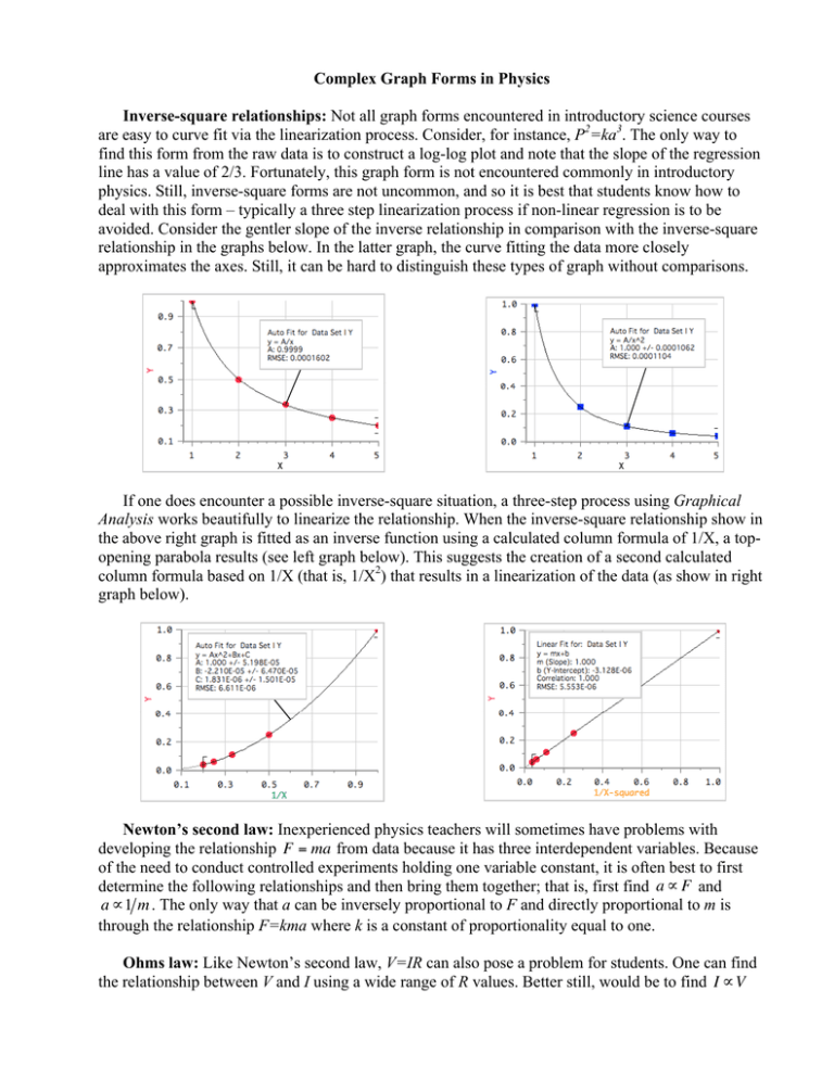
Complex Graph Forms in Physics
Inverse-square relationships: Not all graph forms encountered in introductory science courses
are easy to curve fit via the linearization process. Consider, for instance, P2=ka3. The only way to
find this form from the raw data is to construct a log-log plot and note that the slope of the regression
line has a value of 2/3. Fortunately, this graph form is not encountered commonly in introductory
physics. Still, inverse-square forms are not uncommon, and so it is best that students know how to
deal with this form – typically a three step linearization process if non-linear regression is to be
avoided. Consider the gentler slope of the inverse relationship in comparison with the inverse-square
relationship in the graphs below. In the latter graph, the curve fitting the data more closely
approximates the axes. Still, it can be hard to distinguish these types of graph without comparisons.
If one does encounter a possible inverse-square situation, a three-step process using Graphical
Analysis works beautifully to linearize the relationship. When the inverse-square relationship show in
the above right graph is fitted as an inverse function using a calculated column formula of 1/X, a topopening parabola results (see left graph below). This suggests the creation of a second calculated
column formula based on 1/X (that is, 1/X2) that results in a linearization of the data (as show in right
graph below).
Newton’s second law: Inexperienced physics teachers will sometimes have problems with
developing the relationship F = ma from data because it has three interdependent variables. Because
of the need to conduct controlled experiments holding one variable constant, it is often best to first
determine the following relationships and then bring them together; that is, first find a ∝ F and
a ∝1 m . The only way that a can be inversely proportional to F and directly proportional to m is
€
through the relationship F=kma where k is a constant of proportionality equal to one.
€
€
Ohms law: Like Newton’s second law, V=IR can also pose a problem for students. One can find
the relationship between V and I using a wide range of R values. Better still, would be to find I ∝V
€
and, separately, I ∝ R . Then, combine the relationships to get V=kIR where data will show that k has
a value of unity.
Thin lens formula: The thin lens formula, 1/f = 1/di+1/do, can pose considerable difficulty as far
€
as graphing
and linearization is concerned. An optician’s “trick” can be used to simplify the process.
Require students to use diopters, not distances, in all their experimental measurements involving the
optical bench. Diopters are the inverses of distances that are expressed first in meters. For instance, a
lens has a focal length of 20cm or 0.2m. This means that the “strength” of the lens expressed in
diopters is 1/0.2 or 5. Plotting all measurements in diopters when working on an optical bench results
in an easy discovery of the thin lens formula. The data the students collect will be clearly linear (not
proportional). The y-intercept when plotting 1/di versus 1/do (both expressed in diopters) turns out to
be 1/f (similarly expressed in diopters) that can be related to one of the parameters of the system
under study. People commonly encounter diopters when they ask to see their eyeglass or contact
prescriptions. A diopter value of -3 represents a negative (concave) lens of strength 3; a diopter value
of +2 represents a positive (convex) lens of strength 2.
Parallel resistance formula: The parallel resistance formula, 1/Rt = 1/R1 + 1/R2 + 1/R3 + …, can
be difficult to derive using resistance values even when using only two resistors. Like the use of
diopters above, when working with parallel circuit equivalent resistances, use mhos. A mho is an
inverse ohm. A graph of mhos results in a linear fit, the constant of proportionality having a physical
meaning that students should be able to relate to one of the parameters of the system under study.
Best-fit formula: Though introductory physics students will rarely see the root mean square error
(RMSE) formula:
RMSE =
∑ ( f (x ) − y )
i
2
i
n
its value can be used to determine which type of a fit (say linear versus power function) is better.
RMSE represents the cumulative deviation of specific data points, yi, from a calculated regression
form expressed as f(xi ). The vertical separation between a point and the best-fit form is squared to
€
remove + and – values representing deviations below and above the regression equation respectively.
They are then averaged and the square root is taken. Consider the following graphs of the same data.
Which graph represents a regression solution that best fits the data? The answer can be found in
the RMSE. The first graph above shows a data set fit with a linear function; the second graph above
shows the same data set fit with a parabolic (second-order power) function. The linear fit has an
RMSE of 0.4596; the power fit has an RMSE of 0.4507. The smaller the value of the RMSE (when
using the same data) suggests the better fit. So, for these data, a power fit is slightly better than a
linear fit (assuming there is no physical model with which to concern ourselves). Physical models
always take precedence over mathematical models.