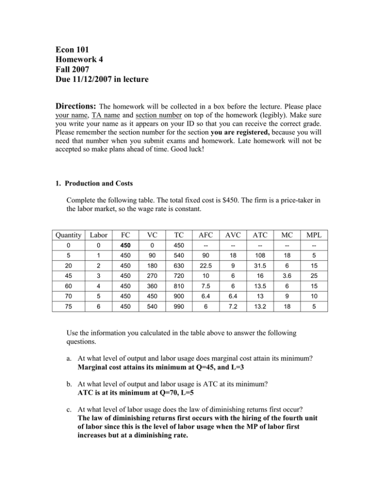
Econ 101
Homework 4
Fall 2007
Due 11/12/2007 in lecture
Directions: The homework will be collected in a box before the lecture. Please place
your name, TA name and section number on top of the homework (legibly). Make sure
you write your name as it appears on your ID so that you can receive the correct grade.
Please remember the section number for the section you are registered, because you will
need that number when you submit exams and homework. Late homework will not be
accepted so make plans ahead of time. Good luck!
1. Production and Costs
Complete the following table. The total fixed cost is $450. The firm is a price-taker in
the labor market, so the wage rate is constant.
Quantity
Labor
FC
VC
TC
AFC
AVC
ATC
MC
MPL
0
0
450
0
450
--
--
--
--
--
5
1
450
90
540
90
18
108
18
5
20
2
450
180
630
22.5
9
31.5
6
15
45
3
450
270
720
10
6
16
3.6
25
60
4
450
360
810
7.5
6
13.5
6
15
70
5
450
450
900
6.4
6.4
13
9
10
75
6
450
540
990
6
7.2
13.2
18
5
Use the information you calculated in the table above to answer the following
questions.
a. At what level of output and labor usage does marginal cost attain its minimum?
Marginal cost attains its minimum at Q=45, and L=3
b. At what level of output and labor usage is ATC at its minimum?
ATC is at its minimum at Q=70, L=5
c. At what level of labor usage does the law of diminishing returns first occur?
The law of diminishing returns first occurs with the hiring of the fourth unit
of labor since this is the level of labor usage when the MP of labor first
increases but at a diminishing rate.
d. When output is equal to zero units, why does the firm still incur costs in the short
run? Explain your answer.
In the short run, the firm still incurs costs even though its production is equal
to zero units because it still has fixed costs. It cannot get rid of its capital
instantaneously so it will continue to have these costs even though it is not
producing any output.
e. As output increases, why does AVC first decrease, but then eventually increase?
Explain your answer.
AVC eventually increases due to diminishing returns to labor: as additional
units of labor are hired the amount of capital per unit of labor decreases
until eventually the additional units of labor are less productive and hence,
this leads to rising average variable costs of production.
f. Suppose the price of output is $20, fill in the following table using the
information you gathered in the above table.
Quantity
0
5
20
45
60
70
75
MC
--18
6
3.6
6
9
18
TR
--100
400
900
1200
1400
1500
TC
450
540
630
720
810
900
990
Profit = TR - TC
-450
-440
-230
180
390
500
510
2. Perfect Competition
Consider a competitive industry with a large number of firms. Assume that all the
firms have identical cost functions. Suppose that initially the demand curve for this
industry is given by Q = 52 – P where Q is the market quantity and P is the market
price. Furthermore an individual firm’s total cost and marginal cost are given by the
following equations:
TC = q2 + 1
MC = 2*q
where q is the quantity supplied by the firm.
a. What is the breakeven price for this firm?
ATC is at its minimum when ATC=MC, q=1, ATC=MC=2. So the breakeven
price for this firm is 2.
b. At the long-run profit maximizing level of output for the firm (i.e. that level of
output where MR = MC = min ATC), what will be the equilibrium output in this
industry?
The equilibrium level of output in the industry can be found by using the
market price of 2 in the market demand curve: thus, P = 52- Q gives us Q =
50.
c. What will be the equilibrium output of each firm in the long-run if each firm is
identical and each firm is profit maximizing?
q=1
d. What will be the equilibrium number of firms in this industry in this long-run
equilibrium?
The equilibrium number of firms in this industry will equal the total level of
production in the market divided by the level of production of a single firm.
At a price of 2, we know that the total production in the market is 50 units
since Q = 52 – P. And, if each firm produces one unit then it will take fifty
firms to produce 50 units.
e. Now suppose the government levies an excise tax of $2 on consumption of this
good. What will be the equilibrium number of firms? What will be the long-run
equilibrium price?
The market demand function becomes: Q=50-P when the excise tax is
imposed on consumers. Since the cost functions have not changed, the longrun equilibrium price remains 2. The number of firms is equal to the
equilibrium market quantity divided the individual firm’s level of production
or 48/1 or 48 firms.
f. Return to the original situation and now suppose that due to environmental
legislation, the fixed cost of production in every firm increases from 1 to 4. What
is the new total cost function? (Marginal cost remains the same).
TC = (q)2 + 4.
g. Suppose the market price is equal to $2 per unit. How do short-run profits change
due to the environmental legislation in part (f)? To answer this question you will
first want to figure out the profit maximizing level of output for the firm, then
check to make sure that the price of $2 is sufficient to cover the firm's AVC since
the firm will choose to shut-down in the short run if it cannot cover its AVC.
Then, if the firm does produce you can figure out the firm's short-run profits by
calculating the difference between its total revenue and its total cost.
In the short run, equilibrium price, and therefore the MR, will still be $2 and
the equilibrium output for a representative firm will be 1 unit. The AVC cost
of producing one unit is equal to 1 and the market price is greater than this
so the firm will choose to produce in the short run since it is covering its
variable cost of production. The firm's total revenue is equal to 2 while its
total cost is equal to 5, so the firm is making a negative economic profit, or a
loss, of 3 in the short run.
h. What do you anticipate will happen in the long-run in this market and what will
be the effect of this change on long-run profits? In your answer make sure you
identify the level of long-run profits for a representative firm, the long-run level
of output for a representative firm, the long-run equilibrium price level, the
market level of output, and the number of firms now producing in this market.
Since firms are making losses in the short run, one can expect the exiting of
firms in the long-run until economic profits return to 0. The exiting of firms
will cause the market price of the good to rise until it reaches the breakeven
point at a price of 4 where each remaining firm is producing 2 units of
output. At a price of 4 there will be 48 units of the good produced by 24
firms. Thus, relative to the initial situation 26 firms will have exited the
market.
To see where these answers come from here is a more detailed description:
Recall that in the long run each firm will produce at its breakeven point
where its ATC curve intersects its MC curve. Thus, to find the ATC curve
you will need to divide TC/Q to get ATC = q + (4/q). Setting this equal to MC
you will have q + 4/q = 2q. Solving for q you will get q = 2. Plugging q = 2
into the MC equation you can calculate the MC as equal to 4. This implies
that the market price is also 4. Using this market price and the market
demand equation you can calculate the market quantity as Q = 48.
equilibrium number of firms is equal to the equilibrium market quantity
divided by the level of production of a representative firm or 48/2 = 24 firms.
3. Income effect and substitution effect
Sally only consumes bread (x) and soda (y). Her indifference curves take the form
x*y = c where x is the number of units of bread, y is the number of units of soda and
c is the total level of utility. Sally’s income is $16. When the price of bread is $4
(Px=$4) and the price of soda is $1 (Py=$1), Sally’s optimal choice is on indifference
curve x*y = 16.
a. Fill in the following table based upon the equation xy = 16 where x is the number
of units of bread and y is the number of units of soda.
X
1
2
4
Y
16
8
4
8
16
2
1
b. Draw the graph placing bread on the horizontal axis and soda on the vertical axis.
How many units of bread and sodas does Sally consume given these prices? What
is her MRS between bread and soda at her optimal consumption bundle?
Sally will consume 2 units of bread and 8 units of sodas. Her MRS between
bread and soda equals the price ratio=4
Now the price of bread falls to $1. Sally’s new optimal choice is on indifference
curve x*y=64.
c. Fill in the following table based upon the equation xy = 64 where x is the number
of units of bread and y is the number of units of soda.
X
1
2
4
8
16
32
64
Y
64
32
16
8
4
2
1
d. What is Sally’s optimal consumption bundle under the new prices? And what is
her MRS between bread and soda at the new optimal consumption bundle? (Hint:
you may want to draw in the new budget line and the new indifference curve on
your original graph.)
At the new prices, Sally will consume 8 units of bread and 8 units of sodas.
Her MRS between bread and soda equals the price ratio=1.
e. What are the substitution effect and income effect for the change in Sally’s
consumption of bread? Illustrate them on your graph, and calculate the change in
bread consumption due to the substitution effect and the change in bread
consumption due to the income effect.
The change from point A to B is substitution effect. The change from point B
to C is income effect. For bread, substitution effect=4-2=2, income effect=84=4
f. Is bread a normal good or an inferior good for Sally? Is soda a normal good or an
inferior good for Sally?
They are both normal goods.
Soda
16
A
C
8
B
4
2
4
8
16
Bread