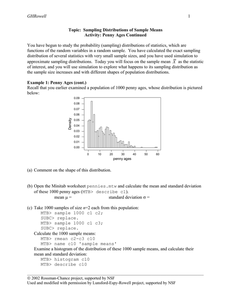
GHRowell
1
Topic: Sampling Distributions of Sample Means
Activity: Penny Ages Continued
You have begun to study the probability (sampling) distributions of statistics, which are
functions of the random variables in a random sample. You have calculated the exact sampling
distribution of several statistics with very small sample sizes, and you have used simulation to
approximate sampling distributions. Today you will focus on the sample mean X as the statistic
of interest, and you will use simulation to explore what happens to its sampling distribution as
the sample size increases and with different shapes of population distributions.
Example 1: Penny Ages (cont.)
Recall that you earlier examined a population of 1000 penny ages, whose distribution is pictured
below:
0.09
0.08
0.07
Density
0.06
0.05
0.04
0.03
0.02
0.01
0.00
0
10
20
30
40
50
60
penny ages
(a) Comment on the shape of this distribution.
(b) Open the Minitab worksheet pennies.mtw and calculate the mean and standard deviation
of these 1000 penny ages (MTB> describe c1).
mean  =
standard deviation  =
(c) Take 1000 samples of size n=2 each from this population:
MTB> sample 1000 c1 c2;
SUBC> replace.
MTB> sample 1000 c1 c3;
SUBC> replace.
Calculate the 1000 sample means:
MTB> rmean c2-c3 c10
MTB> name c10 'sample means'
Examine a histogram of the distribution of these 1000 sample means, and calculate their
mean and standard deviation:
MTB> histogram c10
MTB> describe c10
_____________________________________________________________________________________
 2002 Rossman-Chance project, supported by NSF
Used and modified with permission by Lunsford-Espy-Rowell project, supported by NSF
GHRowell
2
Comment on the shape and record these values:
shape:
mean of sample means:
standard deviation of sample means:
(d) Repeat (b) with samples of size n=5. [Hints: Use c2-c6 to store the 1000 samples, then put
the sample means into c10.] Comment on the shape and record these values:
shape:
mean of sample means:
standard deviation of sample means:
(e) How has the shape of the (approximate) sampling distribution changed as the sample size
increased? How has the mean of the sample means changed? How about the standard
deviation?
shape:
mean:
standard deviation:
The following histograms reveal the (approximate) sampling distributions of the sample mean
X for sample sizes of n=10 and n=30:
100
100
std dev = 3.266
mean = 12.216
Frequency
mean = 12.173
y
c
n
e
u
q
e
r
F
50
0
std dev = 1.745
50
0
0
5
10
15
sample means (n=10)
20
25
10
15
20
sample means (n=30)
(f) What do these simulation reveal about the shape of the sampling distribution of X as the
sample size increases?
_____________________________________________________________________________________
 2002 Rossman-Chance project, supported by NSF
Used and modified with permission by Lunsford-Espy-Rowell project, supported by NSF
GHRowell
3
(g) What do these simulation reveal about the mean of the sampling distribution of X as the
sample size increases?
(h) What do these simulation reveal about the standard deviation of the sampling distribution of
X as the sample size increases?
Example 2: Grade Point Averages (cont.)
Recall that you have studied the grade point averages of Oliver, who has a .5 probability of an A,
.3 of a B, and .2 of a C, independently from course to course. You previously found the exact
distribution of Oliver’s grade point average (sample mean grade points) in a sample of n=2
courses, and you used simulation to approximate this distribution in a sample of n=4 courses.
Now you will simulate the probability (sampling) distribution of the sample mean X in a sample
of n=10 courses (that Oliver might take in one year) and in a sample of n=40 courses (that Oliver
might take in his college career).
(a) Open a new Minitab worksheet (File> New), and enter the values 4, 3, 2 into c1 and their
respective probabilities .5, .3, .2 into c2. Simulate 1000 repetitions of Oliver’s grade points
in a sample of 10 courses:
MTB> random 1000 c11-c20;
SUBC> discrete c1 c2.
Convince yourself that the distribution in any course comes close to 50% A’s, 30% B’s, and
20% C’s:
MTB> tally c11-c20
Calculate the sample mean grade points for these 1000 samples:
MTB> rmean c11-c20 c21
MTB> name c21 'sample means'
Examine a histogram and descriptive statistics:
MTB> histogram c21
MTB> describe c21
Comment on the shape and record these values:
shape:
mean of sample means:
standard deviation of sample means:
(b) Is the mean of these sample means close to  (the mean grade points in any one course),
which you previously found to equal 3.3?
(c) The standard deviation of these sample means is about how many times smaller than  (the
standard deviation of grade points in any one course)?
_____________________________________________________________________________________
 2002 Rossman-Chance project, supported by NSF
Used and modified with permission by Lunsford-Espy-Rowell project, supported by NSF
GHRowell
4
(d) Repeat (a), (b) and (c) by simulating 1000 repetitions of a 40-course college career for
Oliver. Comment particularly on how the shape, mean, and standard deviation compare
between the n=40 and n=10 cases.
shape:
mean of sample means:
standard deviation of sample means:
comparison with n=10 case:
Example 3: Random Lunch Times (cont.)
Re-consider Mary, with her lunch arrival time following a uniform distribution between 0 and 60
minutes after noon (with mean =30 and standard deviation =17.32). Use simulation to
investigate the distribution of her sample mean arrival time in a sample of size n=2. [Hint: Use
the uniform subcommand to the random command.] Then repeat for sample sizes of n=5 and
n=20. Record your findings in the table below.
sample size
2
5
20
shape of samp. dist.
mean of sample means
std. dev. of sample means
Example 4: Birth Weights (cont.)
Recall that birthweights of babies born in the U.S. follow a normal distribution with mean 3250
ounces and standard deviation 550 ounces. Use simulation (normal subcommand to random
command) to investigate the distribution of sample mean birthweights in a sample of size n=2.
Then repeat for sample sizes of n=5 and n=20. Record your findings in the table below.
sample size
2
5
20
shape of samp. dist.
mean of sample means
std. dev. of sample means
Your simulation analyses should convince you that the following results (known as the Central
Limit Theorem) about the sampling distribution of a sample mean X are reasonable:
 The mean of the sampling distribution of X equals the population mean , regardless of the
sample size or the population distribution.
 The standard deviation of the sampling distribution of X equals the population standard
deviation  divided by the square root of the sample size, regardless of the population
distribution.
 The shape of the sampling distribution of X is approximately normal for large sample sizes,
regardless of the population distribution, and it is normal for any sample size when the
population distribution is normal.
_____________________________________________________________________________________
 2002 Rossman-Chance project, supported by NSF
Used and modified with permission by Lunsford-Espy-Rowell project, supported by NSF