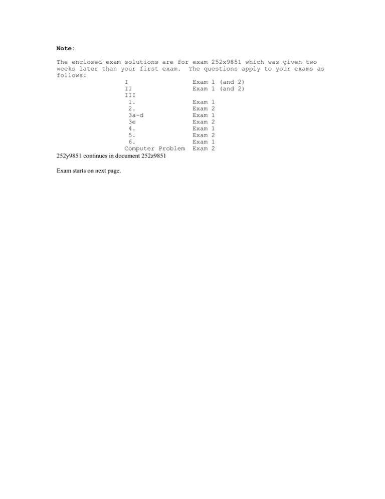
Note:
The enclosed exam solutions are for exam 252x9851 which was given two
weeks later than your first exam. The questions apply to your exams as
follows:
I
Exam 1 (and 2)
II
Exam 1 (and 2)
III
1.
Exam 1
2.
Exam 2
3a-d
Exam 1
3e
Exam 2
4.
Exam 1
5.
Exam 2
6.
Exam 1
Computer Problem Exam 2
252y9851 continues in document 252z9851
Exam starts on next page.
10/23/98 252y9851
ECO252 QBA2
FIRST HOUR EXAM
October 17, 1998
Name
Show your work!
I. (14 points) Do all the following.
x ~ N 1.5,8
1.
30  1.5 
 1  1.5
z
P1  x  30  P
  P 0.06  z  3.56 
8 
 8
 P 0.06  z  0  P0  z  3.56   .0239  .4998  .5237
5  1.5 
  5  1.5
z
2. P 5  x  5  P
  P 0.81  z  0.44 
8
8 

 P0.81  z  0  P0  z  0.44   .2910  .1700  .4610
9  1.5 
  3  1.5
z
3. P3  x  9  P
  P0.19  z  0.94 
8
8 

 P0  z  0.94   P0  z  0.19   .3264  .0753  .2511
 0  1.5 

4. Px  0  P z 
  P z  0.19 
8


 P0.19  z  0  Pz  0  .0753  .5000  .5753
1.5  1.5 
  7  1.5
z
5. P 7.0  x  1.5  P
  P 1.06  z  0   .3554
8
8


6.
A symmetrical interval about the mean with 63% probability.
We want two points x .1850 and x.8150 , so that Px.1850  x  x .8150   .6300 . From the
diagram, if we replace x by z, P0  z  z.1850   .3150 . The closest we can come is
P0  z  0.90   .3159 . So z.1850  0.90 , and x    z.1850  1.5  0.908  1.5  7.2 , or –5.7 to 8.7.
7.
x.045
We want a point x .045 , so that Px x .045   .045 . From the diagram, if we replace x by z,
P0  z  z.045   .455 . The closest we can come is P0  z  1.70   .4554 . So z.045  1.70 , and
x    z.045  1.5  1.708  1.5  13 .6 , or 15.1 .
2
10/23/98 252y9851
II. (6 points-2 point penalty for not trying part a.) Show your work!
Samples of five automobiles from one manufacturer and six automobiles from a second
manufacturer were tested for top speeds. These are listed below. Assume that we were sampling from a
normal distribution.
Manufacturer 1
Manufacturer 2
Automobile Speed Automobile Speed
1
110
1
115
2
135
2
130
3
125
3
140
4
185
4
190
5
130
5
135
6
142
Note that x 2  142 , s 2  25.4165
a.
Compute the sample variance, s1 , of the top speed of automobiles for the first manufacturer.
Show your work.(3)
Solution:
x1
 x  685  137

n
x

5
97075  5137 2
n 1
4
 807 .5 or s1  28.4165 .
s12
2
 nx1 2

Manufacturer
1
2
3
4
5
Total
x (Speed)
110
135
125
185
130
685
x2
12100
18225
15625
34225
16900
97075
.
b. Compute a 99% confidence interval for the mean top speed, 1 , of automobiles for the first
manufacturer.(3)
Solution: From the problem statement  .01 . From page 10 of the syllabus supplement, if the
population variance is unknown   x  t  s x and t n21  t .4005  4.604 .
2
s x1 
s1
n

807 .5 28 .4165

 12 .7083 . So 1  137  4.604 12.7083   137  58.51 or 76.49 to 195.51.
5
5
3
10/23/98 252y9851
III. Do at least 3 of the following 6 Problems (at least 10 each) (or do sections adding to at least 30 points Anything extra you do helps, and grades wrap around) . Show your work!
1. Using the data from the previous problem (page 2.), test the hypothesis that the population mean, 1 , for
the first manufacturer is 135 at the 99% confidence level using:
a. A test ratio (2)
b. Critical values (2)
c. A confidence interval (2)
d. Find an approximate p-value for the null hypothesis. (1)
e. Now find a 95% confidence interval for the standard deviation.(3)
Solution: From page 10 of the Syllabus Supplement:
Interval for
Confidence
Hypotheses
Test Ratio
Critical Value
Interval
Mean (
known)
  x  z  x
Mean (
unknown)
  x  t  sx
2
2
DF  n  1
H 0 :   135
H 1 :   135
H0 :   0
z
H1 :    0
H 0 :   0
H1:   0
t
x  0
x
x  0
x cv   0  z 2  x
x cv   0  t  2 s x
sx
4
10  135 , DF  n  1  4,   .01, tn 1  t .005
 4.604
2
From the previous page: x1  137 and s x1 
s1

807 .5 28 .4165

 12 .7083 .
5
5
n
x  10 137  135

 0.1574 . This is in the 'accept region'
a. Test Ratio: t 
s x1
12 .7083
between -4.604 and +4.604, so accept H 0 .
b. Critical Value: xcv  10  t sx1  135  4.604 12.7083   135  58.51 or 76.5
2
to 193.5. This includes x1  137 , so accept H 0 .
c. Confidence Interval: 1  x1  t  s x1  137  4.604 12.7083   137  58.51
2
or 78.5 to 195.5. This includes 10  135 , so accept H 0 .
4
 0.134 , so that, if this were a 1-sided test, we could say
d. From the t table t = 0.1574 is smaller than t .45
pvalue  45 . Since this is a 2-sided test, we double p-value, and say pvalue 90 .
e. From page 1 of the Syllabus Supplement:
 n  1 s 2
 2
2
Since 
2
 .025 and 1  
2
4807 .5   2  4807 .5
1
11 .1433
0.2158
17.025   1  122 .342 .
2 
 n  1 s 2
2
1
4 
2 4 
and  .975 . So
 .975 , look up  .2025
. DF  n  1  4 and   .05 .

2
n  1s12
 .2025
  12 
n  1s12
 .2975
or
or 289.86   12  14967.56 . Finally, taking square roots,
4
10/23/98 252y9851
2. Repeating the data from the previous problem:
Manufacturer 1
Automobile Speed
1
110
2
135
3
125
4
185
5
130
Manufacturer 2
Automobile Speed
1
115
2
130
3
140
4
190
5
135
6
142
Note that x 2  142 , s 2  25.4165
Test the hypothesis that cars produced by the second manufacturer have higher top speeds than
those produced by the first manufacturer by comparing means using:
a. A test ratio (3)
b. Critical values (2)
c. A confidence interval (2)
d. Find an approximate p-value for the null hypothesis. (1)
e. Now find a 95% confidence interval for the ratio,
1
, of standard deviations.(3)
2
Note: You may assume either (i) that population variances are the same for the two parent populations or
(ii) that they are not equal, but if you assume that they are not equal part a) is 5 points and b) and c) are 3
points each. So, indicate what you assume.
f. Do a test to see if the which of the two assumptions is correct. (2)
Solution: From page 10 of the Syllabus Supplement:
Difference
H 0 :   0 *
  d  t  2 sd
between Two
H 1:   0
1
1
Means (
sd  s p

  1   2
n1 n2
Unknown,
DF

n

n

2
1
2
Variances
Assumed equal)
2
s12 s22

n1 n2
sd 
DF 
 s12 s22 
  
n

 1 n2 
sˆ 2p 
H 0 :   0 *
  d  t  sd
Difference
Between Two
Means(
Unknown,
Variances
Assumed
Unequal)
t
t
H 1:   0
  1   2
d cv   0  t  2 sd
d 0
sd
n1  1s12  n2  1s22
n1  n2  2
d cv   0  t  2 sd
d  0
sd
2
   
s12
2
n1
n1  1
s 22
2
n2
n2  1
Recall that. x1  137 , s1  28.4165 , n1  5 and x 2  142 , s 2  25.4165 , n 2  6
H0 :    0
d  x1  x2  137  142  5
(i)Assume
sˆ p 
 12
  22
n1  1s12  n2  1s22
n1  n2  2
1
1


n1 n2

428.41652  525.41652
9
717 .7758  1  1 
 263 .1845  16 .2230
  1   2  0
(ii)Assume  12   22
 717 ,7758  26 .7913
sd  s p
H1 :    0
5
6
s12 28 .4165 2

 161 .4995
n1
5
s22 25 .4165 2

 107 .6156
n2
6
2
2
If we sum these s1  s2 =269.1151.
n1
n2
10/23/98 252y9851
5
Equal variances
Unequal variances
sd  16.2230
DF  n1  n2  2  5  6  2  9
s12 s22

n1 n2
sd 
 269 .1151  16 .4047
DF 
 s12 s22 



n

 1 n2 
   
s12
2
n1
n1  1

2
s 22
2
n2
n2  1
269 .1151 2
161 .4995 2  107 .6156 2
4
 8.1959
5
Use 8 degrees of freedom.
t
a)
d  0
50

 0.3082
sd
16 .2230
9
t  t.025
 2.262 So accept H 0
2
b)
d cv   0  t  2 sd
 0  2.262 16 .2230 
 36.70 Accept H 0
c)
  d  t  sd
2
 5  36.70
t
a)
d  0
50

 0.3047
sd
16 .4074
8
t  t.025
 2.306 so accept H 0
2
b) d cv   0  t  sd
2
 0  2.306 16 .4074 
 37.84 Accept H 0
c)
  d  t  sd
2
 5  37.84
The interval includes 0, so accept H 0 .
The interval includes 0, so accept H 0 .
9
9
d) t.35
 0.398 t.40
 0.261and our
t  0.3082 . So for a 1-sided test we would get
.35  p  value  .40 , but this is a 2-sided test, so
.70  p  value  .80 .
8
8
d) t.35
 0.399 t.40
 0.262 and our
t  0.3047 . So for a 1-sided test we would get
.35  p  value  .40 , but this is a 2-sided test, so
.70  p  value  .80 .
6
10/23/98 252y9851
e) From page 11 of the Syllabus Supplement:
Interval for
Confidence
Hypotheses
Interval
Ratio of
 22 s22 DF1 , DF2
H 0 :  12   22

F

Variances
12 s12 .5 .5 2 
H 1 :  12   22
1
DF1 , DF2
F1  2
 DF1 , DF2
DF1  n1  1
F 2
Test Ratio
Critical Value
F DF1 , DF2 
s12
s22
and
DF2  n2  1
F
DF2 , DF1
 2

.5  .5  2    or
1  
2

s22
 2
s1

2
 12 s12 ( n2 1, n1 1)
1
 22 s22 DF1 , DF2 means s1


F
as is explained in “Confidence Limits and

F

12 s12 .5 .5 2 
s 22 Fn1 1, n2 1  22 s 22 2
2
Hypothesis Tests for Variances”. So
5, 4
F.025
 9.36 and
1.25
e)
s12
s 22

28 .4165 
25 .4165 2
2
s12
s 22
2
1
s2
( n 1, n1 1)
1
1
2
n1 1, n2 1   2  s 2 F 2
F
2
2
4, 5
 7.39 ,
. Now F.025
2
 1.250 , so
s12
s 22
 12 s12 (5, 4)

4,5   2  s 2 F.025 becomes
F.025
2
2
1
2
2
1
 12  1.259.36  . So 0.169  12  11 .7 .
7.39  2
2
H 0 :  12   22
H 1 :  12
s2
F 5, 4,  22
s1


2
2
is tested by using F 4,5 
25 .4165 2
28 .4165 2
s12
s 22

28.4165 2
25.4165 2
4, 5
 7.39 and
 1.25 against F.025
5, 4
 9.36 . The second test is unnecessary due to the fact that
 0.800 against F.025
all F s on the table are above 1. Since in both tests, the F ratios are below the table values, accept H 0 .
7
10/23/98 252y9851
3. Data from section II is repeated below.
Manufacturer 1
Manufacturer 2
Automobile Speed Automobile Speed
1
110
1
115
2
135
2
130
3
125
3
140
4
185
4
190
5
130
5
135
6
142
Note that x 2  142 , s 2  28.4165
a. Test that the population mean,  2 (second sample), is 135 assuming that the parent population is
normally distributed and that the sample of six is taken from a population of 40. (3)
b. Drop the assumption that the parent distribution is normal ( and that the population size is 50) and figure
out a confidence level for the confidence interval ( 130   142 ) (3)
c. Put a p-value on the statement that the median is 129, again assuming that the distribution is not normal.
(2)
d. Looking at your result in c, would you reject the hypothesis that the median is 129 at the 90% confidence
level? Explain. (1)
e. Test the hypothesis that cars produced by the second manufacturer have higher top speeds than those
produced by the first manufacturer by comparing medians assuming that the parent populations are not
normal. (5)
Solution:
a)
H 0 :  2  135 H1 :  2  135
5
5
 2.571 .
10  135 , DF  n  1  5,   .01 or .05, tn 1  t .005
 4.032 or t .025
2
x 2  142 and s x 2 
(i) Test Ratio: t 
s2
n2
N 2  n 2 25 .4165

N 2 1
6
40  6
 9.6883 .
40  1
x   20 142  135

 0.7225 . This is in the 'accept region'
sx2
9.6883
between  t5  and ,  t5  so accept H 0 .
2
2
or (ii) Critical Value: xcv  10  t sx1  135  t5 9.6883  . This includes x 2  142 , so accept H 0 .
2
2
or(iii) Confidence Interval:  2  x 2  t  s x1  137  t 52 9.6883  . This includes 10  135 , so accept H 0 .
2
b) If we put our data in order, we get: ( x1 is the original numbers in order, r1 is their rank.)
If we look only at x 2 , the confidence interval ( 130   142 ) is wrong if 5 or
x1
r1
x 2 r2
110
125
1
3
115
130
2
4.5
130 4.5 135
135 6.5 140
185 10 142
190
25
6.5
8
9
11
41
more numbers are above the median or 5 or more numbers are below the
median. From the binomial table for n  6 and p  .5 we find that
Px  5  Px  1  .10938 . The probability we want is the probability of
one of two different events with probability .10938, so our significance level is
.21878 and the confidence level is 1 - .21878 =.78124.
8
10/23/98 252y9851
c) To test the statement H 0 :  129 , note that in x 2 there are five numbers above 129. If 129 is the
median the chance that any one number is above the median is .5. Since we expect that 3 out of 6 will be
above the median, and because this is a 2-sided test, the p-value is
2Px  5  21  Px  4  21  .89062   .21876 .
d) Since our significance level is 10% and the p-value is above that, accept H 0 :  129 .
e) H 0 : 1  2 H 1 : 1   2 Using Table 5 for the Wilcoxon Rank Sum test for independent samples, if W
= 25 ( This is the smaller rank sum on the bottom of page 7 in this document), its p-value is .214. If the
significance level is 5% or 10% we accept H 0 . If we use Table 6b for a 5% one-tailed test, we find that the
accept region is between 20 and 40, so accept H 0 .
Exam solution continues in 252z9851.doc
9