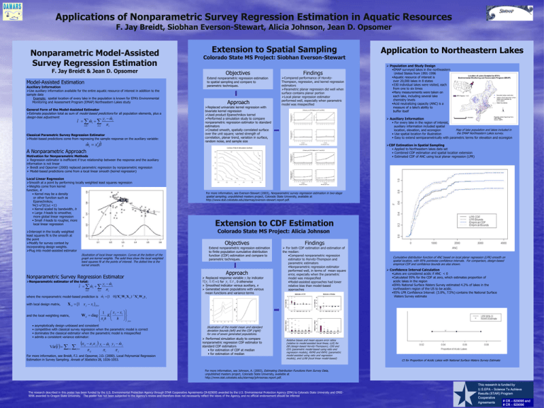
Applications of Nonparametric Survey Regression Estimation in Aquatic Resources
F. Jay Breidt, Siobhan Everson-Stewart, Alicia Johnson, Jean D. Opsomer
Nonparametric Model-Assisted
Survey Regression Estimation
F. Jay Breidt & Jean D. Opsomer
Model-Assisted Estimation
Auxiliary Information
Use auxiliary information available for the entire aquatic resource of interest in addition to the
sample data
Example: spatial location of every lake in the population is known for EPA’s Environmental
Monitoring and Assessment Program (EMAP) Northeastern Lakes study
General Form of the Model-Assisted Estimator
Estimate population total as sum of model-based predictions for all population elements, plus a
design-bias adjustment:
y  mˆ
tˆ   mˆ i  
iU
is
i
i
i
Classical Parametric Survey Regression Estimator
Model-based predictions come from regressing the sample response on the auxiliary variable:
ˆ i  xi̂
m
Extension to Spatial Sampling
Colorado State MS Project: Siobhan Everson-Stewart
Objectives
Extend nonparametric regression estimation
to spatial sampling and compare to
parametric techniques.
Approach
Replaced univariate kernel regression with
bivariate kernel regression
Used product Epanechnikov kernel
Performed a simulation study to compare
nonparametric regression estimator to standard
estimators
Created smooth, spatially correlated surface
over the unit square; varied strength of
correlation, planar trend, variation in surface,
random noise, and sample size
Findings
Compared performance of HorvitzThompson, regression, and kernel regression
estimators
Parametric planar regression did well when
surface contains planar portion
Local planar regression estimator
performed well, especially when parametric
model was misspecified
CDF Estimation in Spatial Sampling
• Applied to Northeastern lakes data set
• Combined CDF estimation and spatial location extension
• Estimated CDF of ANC using local planar regression (LPR)
Motivation for Nonparametric Methods
 Regression estimator is inefficient if true relationship between the response and the auxiliary
information is not linear
 Breidt and Opsomer (2000) replaced parametric regression by nonparametric regression
 Model-based predictions come from a local linear smooth (kernel regression)
Extension to CDF Estimation
Objectives
Illustration of local linear regression. Curves at the bottom of the
graph are kernel weights. The solid lines show the local weighted
least squares fit at the points of interest. The dotted line is the
kernel smooth.
Nonparametric Survey Regression Estimator
Nonparametric estimator of the total:
ˆ
ˆt   mˆ i   yi  mi
iU
is
i
ˆ i  [1 0]( Xsi Wsi X si ) 1 Xsi Wsi y s
where the nonparametric model-based prediction is m
Extend nonparametric regression estimation
to finite population cumulative distribution
function (CDF) estimation and compare to
parametric techniques.
Approach
 Replaced response variable yi by indicator
1{ yi  t} =1 for yi  t , 0 otherwise
 Smoothed indicator versus auxiliary, x
 Generated seven populations with various
mean functions and variance terms
Findings
 For both CDF estimation and estimation of
the median:
•Compared nonparametric regression
estimator to Horvitz-Thompson and
parametric estimators
•Nonparametric regression estimator
performed well, in terms of mean square
error, especially when the parametric
model was misspecified
•Model-assisted approaches had lower
relative bias than model-based
approaches
Cumulative distribution function of ANC based on local planar regression (LPR) smooth on
spatial location, with 95% pointwise confidence intervals. For comparison, design-based
empirical CDF and confidence bounds are also shown.
 Confidence Interval Calculation
•Lakes are considered acidic if ANC < 0
•Calculated 95% for the CDF at zero, which estimates proportion of
acidic lakes in the region
•EPA’s National Surface Waters Survey estimated 4.2% of lakes in the
northeastern region of the US to be acidic.
•95% LPR Confidence Interval: (3.0%, 7.5%) contains the National Surface
Waters Survey estimate
X si  [1 x j  xi ] js
and the local weighting matrix,
•
•
•
•
For more information, see Everson-Stewart (2003), Nonparametric survey regression estimation in two-stage
spatial sampling, unpublished masters project, Colorado State University, available at
http://www.stat.colostate.edu/starmap/everson-stewart.report.pdf.
Colorado State MS Project: Alicia Johnson
Intercept in the locally weighted
least squares fit is the smooth at
the point
Modify for survey context by
incorporating design weights.
Plug into model-assisted estimator
with local design matrix,
 Population and Study Design
•EMAP surveyed lakes in the northeastern
United States from 1991-1996
•Aquatic resource of interest is
over 20,000 lakes in 8 states
•330 individual lakes were visited, each
from one to six times
•Many measurements were taken on
each lake, including several lake
chemistry levels
•Acid neutralizing capacity (ANC) is a
measure of a lake’s ability to
buffer itself
 Auxiliary Information
• For every lake in the region of interest,
auxiliary information included spatial
Map of lake population and lakes included in
location, elevation, and ecoregion
the EMAP Northeastern Lakes survey.
• Use spatial location for illustration
• Easy to extend semiparametrically with parametric terms for elevation and ecoregion
A Nonparametric Approach
Local Linear Regression
Smooth at a point by performing locally weighted least squares regression
Weights come from kernel
function, K
• Kernel may be a density
or other function such as
Epanechnikov,
¾(1-u2)I{|u| <1}
• Kernel scaled by bandwidth, h
• Large h leads to smoother,
more global linear regression
• Small h leads to rougher, more
local linear regression
Application to Northeastern Lakes
 1  x j  xi 

Wsi  diag 
K 
 jh  h  js
asymptotically design unbiased and consistent
competitive with classical survey regression when the parametric model is correct
dominates the classical estimator when the parametric model is misspecified
admits a consistent variance estimator:
Vâr tˆ   is  js

ij
  i j  yi  mˆ i y j  mˆ j
 ij
i
j
For more information, see Breidt, F.J. and Opsomer, J.D. (2000). Local Polynomial Regression
Estimation in Survey Sampling. Annals of Statistics 28, 1026-1053.
Illustration of the model mean and standard
deviation bounds (left) and the CDF (right)
for one of seven generated populations.
 Performed simulation study to compare
nonparametric regression CDF estimator to
standard CDF estimators
• for estimation of CDF at median
• for estimation of median
Relative biases and mean square error ratios
(relative to model-assisted local linear, LLR) for
DB (design-based Horvitz-Thompson), CD0 and
CD1 (parametric model-based using ratio and
regression models), RKM0 and RKM1 (parametric
model-assisted using ratio and regression
models), and LLRB (local linear model-based)
CI for Proportion of Acidic Lakes with National Surface Waters Survey Estimate
For more information, see Johnson, A. (2003), Estimating Distribution Functions from Survey Data,
unpublished masters project, Colorado State University, available at
http://www.stat.colostate.edu/starmap/johnsonaa.report.pdf.
The research described in this poster has been funded by the U.S. Environmental Protection Agency through STAR Cooperative Agreements CR-829095 awarded by the U.S. Environmental Protection Agency (EPA) to Colorado State University and CR829096 awarded to Oregon State University. The poster has not been subjected to the Agency's review and therefore does not necessarily reflect the views of the Agency, and no official endorsement should be inferred
This research is funded by
U.S.EPA – Science To Achieve
Results (STAR) Program
Cooperative
# CR – 829095 and
Agreements
# CR – 829096