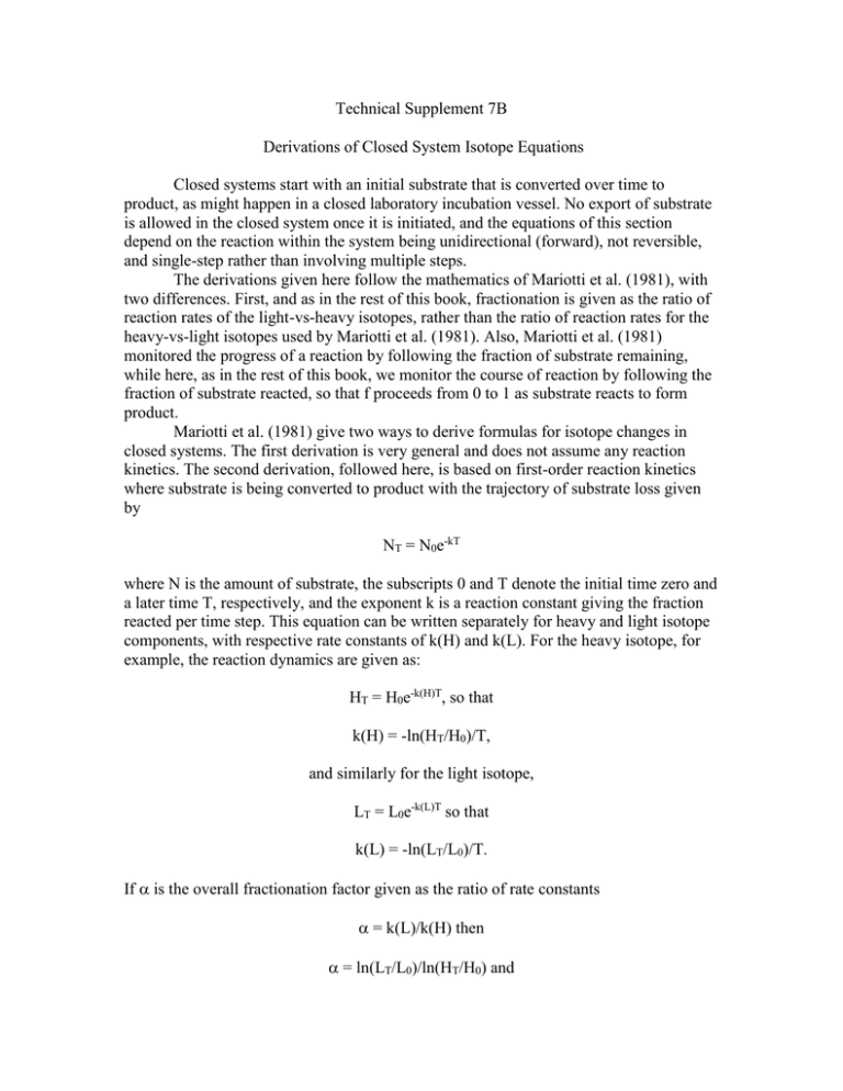
Technical Supplement 7B
Derivations of Closed System Isotope Equations
Closed systems start with an initial substrate that is converted over time to
product, as might happen in a closed laboratory incubation vessel. No export of substrate
is allowed in the closed system once it is initiated, and the equations of this section
depend on the reaction within the system being unidirectional (forward), not reversible,
and single-step rather than involving multiple steps.
The derivations given here follow the mathematics of Mariotti et al. (1981), with
two differences. First, and as in the rest of this book, fractionation is given as the ratio of
reaction rates of the light-vs-heavy isotopes, rather than the ratio of reaction rates for the
heavy-vs-light isotopes used by Mariotti et al. (1981). Also, Mariotti et al. (1981)
monitored the progress of a reaction by following the fraction of substrate remaining,
while here, as in the rest of this book, we monitor the course of reaction by following the
fraction of substrate reacted, so that f proceeds from 0 to 1 as substrate reacts to form
product.
Mariotti et al. (1981) give two ways to derive formulas for isotope changes in
closed systems. The first derivation is very general and does not assume any reaction
kinetics. The second derivation, followed here, is based on first-order reaction kinetics
where substrate is being converted to product with the trajectory of substrate loss given
by
NT = N0e-kT
where N is the amount of substrate, the subscripts 0 and T denote the initial time zero and
a later time T, respectively, and the exponent k is a reaction constant giving the fraction
reacted per time step. This equation can be written separately for heavy and light isotope
components, with respective rate constants of k(H) and k(L). For the heavy isotope, for
example, the reaction dynamics are given as:
HT = H0e-k(H)T, so that
k(H) = -ln(HT/H0)/T,
and similarly for the light isotope,
LT = L0e-k(L)T so that
k(L) = -ln(LT/L0)/T.
If  is the overall fractionation factor given as the ratio of rate constants
 = k(L)/k(H) then
 = ln(LT/L0)/ln(HT/H0) and
 ln(LT/L0) = ln(HT/H0)
Subtract ln(LT/L0) from each side of the previous equation so that
 ln(LT/L0) - ln(LT/L0) = ln(HT/H0) - ln(LT/L0)
For the left side of the equation, let f = fraction of substrate reacted so that 1- f = LT/L0 or
1- f = the fraction of substrate that is not yet reacted, so that:
*ln(1-f) = ln(HT/H0) - ln(LT/L0).
The right side of the equation rearranges to:
ln(HT/H0) - ln(LT/L0) = ln[(HT/H0)/(LT/L0)] = ln[(HT/LT)/(H0/L0)] = ln (RT/R0)
where R is the ratio of heavy to light isotopes = H/L. This yields:
ln(1- f) = ln(RT/R0), or
RT/R0 = (1 - f)(1/

Recognizing that this formula applies to substrate that is being consumed, or residual
substrate (RS), we can substitute the term RRS for RT to show that it is substrate involved
in this equation. The ratio R0 denotes the initial substrate value.
RRS/R0 = (1 - f)(1/
This equation is widely-known in the isotope literature as the Rayleigh equation, and was
derived by John William Strutt who later in life became Lord Rayleigh. This equation
was actually not derived for isotopes, but more generally for distillation of binary
mixtures (Rayleigh 1902). On another note, Mariotti et al. (1981) show that this equation
can be derived independently of the assumption of first order rate constants – see that
paper for details.
The remainder of this section considers ways to manipulate Lord Rayleigh’s
equation to estimate fractionation factors from experimental data. Exact equations are
derived first using the ratio (R) notation, then approximate equations are derived using
the  notation.
Exact Equations with the Ratio Notation
A) Equations for Substrate. Derivations start by recognizing that the RT/R0 term in the
left side of Rayleigh’s equation is closely related to observed  values of substrate that is
being used up, or residual substrate RS:
RS = (RRS/R0 – 1)*1000 so that
RRS/R0 = 1 + RS/1000
Substituting for RRS/R0 and using logarithmic transformations one obtains
ln(1 + RS/1000) = (1/*ln(1 – f)
which is an equation for a straight line with slope = 1/ when measured (x,y) data are
in the form (ln(1 – f), ln(1 + RS/1000)).
However, there are several further steps before these calculations can be used
easily with measured substrate concentration data from lab or field situations. These steps
involve substituting concentration data for the x-term in the (x,y) data, i.e., the term ln(1 f).The mathematics for this substitution are given as follows.
The term ln(1 - f) can be decomposed to
ln(LT/L0) = ln (LT) – ln(L0)
where ln(L0) is a constant, c1, so that
ln(1 + RS/1000) = (1/*(ln(LT) - c1)
Because (1/*c1 is also a constant, c2,
ln(1 + RS/1000) = (1/*ln (LT) - c2
Fortuitously, the light isotope makes up nearly 100% of the total mass of the element for
the common measured H,C,N,O and S isotopes, so that the mass of the light isotope, LT,
is an excellent proxy for the total concentration of the element.
ln(1 + RS/1000) = (1/*ln(concentration) - c2.
This is again the equation for a line with slope (1/, where (x,y) data for substrate
are of the form: (x,y) = (ln(concentration), ln(1 + RS/1000)). Overall, this final result is
very useful, because it allows estimation of fractionation factors in closed systems from
just the isotope values and the concentration values of substrate that is being consumed.
The fractionation factor is derived from the slope of the line as:
 = (1/(slope + 1)) or  = (-1000*slope)/(slope + 1)
B) Equations for the instantaneous product. Products formed from substrate can have a
transient existence in closed systems, if product is continually formed then removed from
a reaction by e.g. precipitation. Newly formed product can be thought of as an
instantaneous product, formed instant-by-instant from substrate. When fractionation
occurs during product formation, the isotope ratio in this instantaneous product (RIP) is
less than that of the substrate, and is obtained by dividing the isotope ratio of the
substrate (RRS) by :
RIP = RRS/
Dividing both sides of this equation by R0 one obtains
RIP/R0 = (1/RRS/R0
Using the Rayleigh equation from above, one can substitute for RRS/R0:
RIP/R0= (1/*(1 - f)(1/
This can be rearranged to
ln(1 + IP/1000) = (1/ – 1)*ln(1 – f) + ln(1/
which is the equation for a straight line with slope = (1/ – 1) when experimental (x,y)
data are in the form (ln(1 – f), ln(1 + IP/1000)) or in the form (ln(concentration), ln(1 +
IP/1000)). The fractionation factor is derived from the slope of the line as:
 = (1/(slope + 1)) or  = (-1000*slope)/(slope + 1)
C) Equations for the Accumulated Product. In addition to the instantaneous product, one
can also examine the cumulative product that builds up over time. For isotope
calculations about accumulated products, a good starting point is that the substrate and
accumulated product in a closed system must add together to equal the initial input. With
this mass balance constraint, one writes the mass balance equation for inputs = outputs as
R0 = RRS*(1-f) + RAP*f
where RAP is the isotope ratio of the accumulated product. This rearranges to:
RAP = [R0 - RRS*(1-f)]/f
Also, to work with experimental data, one can rearrange to:
f *RAP/R0 + (1-f)*RRS/R0= 1 or
f *RAP/R0 = 1 - (1-f)*RRS/R0
If AP = (RAP/R0 -1)*1000, then RAP/R0 = (1+ AP/1000)
Substituting for both RAP/R0 and RRS/R0 one obtains
f*(1+ AP/1000) = 1 – (1-f)*(1-f)(1/ - 1) so that
1 - f*(1 + AP/1000) = (1-f)(1/ and
ln[1 - f*(1 + AP/1000)] = (1/)*ln(1 – f)
This will yield a straight line when (x,y) data are in the form (ln(1 – f), ln[1 - f*(1 +
AP/1000)]) with slope 1/ so that the fractionation factor  = 1/slope.
Approximate Equations with the  Notation
Mariotti et al. (1981) give approximate solutions for isotope values of substrate
and products when  fractionations are small relative to 1000o/oo, as is the usual case.
Closed-system equations that emerge from these approximations are relatively
straightforward and are those shown in Fig. 7.4. The many steps of this more
approximate derivation follow.
A) Equations for Substrate.
The first steps of this more approximate approach work with the relationship
between  and the fractional extent of reaction. One starts again with the Rayleigh
equation which gives the isotope ratio of the substrate at time t (RRS) relative to the initial
substrate isotope value (R0) as:
RRS/R0 = (1 - f)(1/
which transforms to
*ln(1 - f) = ln(RRS/R0),
then focuses on the left term, i.e., *ln(1 - f). If  is the fractionation factor
derived from  and expressed as a positive number in permil units, i.e.,
 = ()*1000 then  = 1 + /1000, and
ln(1- f) = [-/(1000+]*ln(1 - f)
Now we work with the right side of the equation,
*ln(1 - f) = ln(RRS/R0),
i.e., with ln (RRS/R0), using the definition of  to determine values for substrate RRS and
R0 at times T and 0 as
RRS = (1 + RS/1000)*RSTD and
R0 = (1 + 0/1000)*RSTD, so that
ln(RRS/R0) = ln[(1 + RS/1000)/(1 + 0/1000)].
Combining results for the left and right side of the equation
*ln(1 - f) = ln(RRS/R0) we have:
ln[(1 + RS/1000)/(1 + 0/1000)] = [-/(1000+]*ln(1 - f )
Although it is not obvious, the left side of this equation is rather simply related to the
measured RS value when the range in  values is fairly narrow, <20o/oo, and 0 is zero
Mariotti et al. (1981) give the formula that justifies this simplification, such that
ln[(1 + u)/(1 + v)] = u - v
when u and v are small relative to 1. Using this approximation, we find that for  values
in the natural abundance range near 0o/oo,
ln[(1 + RS/1000)/(1 + 0/1000)] = (RS /1000) - (0/1000) = RS /1000
when (Note: if the measured 0 value for the substrate is not zero, isotope values
can be recalculated to refer to this initial input substrate as the reference value, effectively
resetting this 0 value to 0o/oo; Conversion 1 in the printed Appendix to the book shows
how to make this recalculation).
The equation
ln[(1 + RS /1000)/(1 + 0/1000)] = [-/(1000+]*ln(1 - f ) thus simplifies to:
RS = [-1000*/(1000+]*ln(1 - f )
When, as is the usual case,  is small relative to 1000, this further simplifies to:
RS = *-ln(1 - f )
Note that this yields a straight line relationship between ln(1 - f) and RS when the data
are plotted as (-ln(1- f), RS), or alternatively as (-ln(concentration),RS). The slope of the
line gives the fractionation factor, .
B) Equations for the instantaneous product. At any instant in time, the fractionation
between substrate and product formed at that instant (the “instantaneous product”) is the
fractionation factor  so that
INSTANTANEOUS PRODUCT = IP = RS - *-ln(1 - f ) - 
With this equation, the fractionation factor  is given as the slope of a line drawn through
(x,y) points of the form:
(x,y) = (-ln(1-f), IP) or alternatively,
(x,y) = (-ln(concentration), IP)
C) Equations for the Accumulated Product. Derivations here start again from the
standpoint that the substrate and product in a closed system must add together to equal
the initial input. With this mass balance constraint, and assuming that the isotope values
are referenced to the starting substrate so that INPUT = 0o/oo, one writes the mass balance
equation that includes the accumulated product AP:
INPUT = 0 = (1 – f)*RS + fAP so that
AP = ((f – 1)/f)*RS
Using the approximations above that are appropriate when the range of isotope
compositions for substrates or products is 20o/oo or less, we have
RS = *-ln(1 - f)
so that one can write:
AP = *((1 - f)/f)*ln(1 - f)
With this formula for the isotope composition of the accumulated product, the
fractionation factor  is obtained as the slope of the line when (x,y) data are in the form
of:
(x,y) = (((1 - f)/f)*ln(1 - f), AP)
Summary
Although the math given above involves many steps, it yields a good framework
for understanding how fractionation is expressed in both substrates and products in closed
systems. The math is valuable since it shows how fractionation factors can be estimated
from the slopes of lines fit to measured (x,y) data. The equations apply to closed systems
that have single-step, unidirectional reactions. In such systems, the same fractionation
factor should emerge when using data sets for substrate, instantaneous product, or
accumulating product. If examination of these three sets of data produces different
fractionation factors, usually the system is not truly closed, or there are several products
being created from the substrate.
Further Reading
Mariotti, A., J.C. Germon, P. Hubert, P. Kaiser, R. Letolle, A. Tardieux and P. Tardieux.
1981. Experimental determination of nitrogen kinetic isotope fractions: some principles;
illustration for the denitrification and nitrification processes. Plant and Soil 62:413-430.
Rayleigh, Lord. 1902. On the distillation of binary mixtures. The London, Edinburgh and
Dublin Philosophical Magazine and Journal of Science, Series 6, Volume 4:521-537.