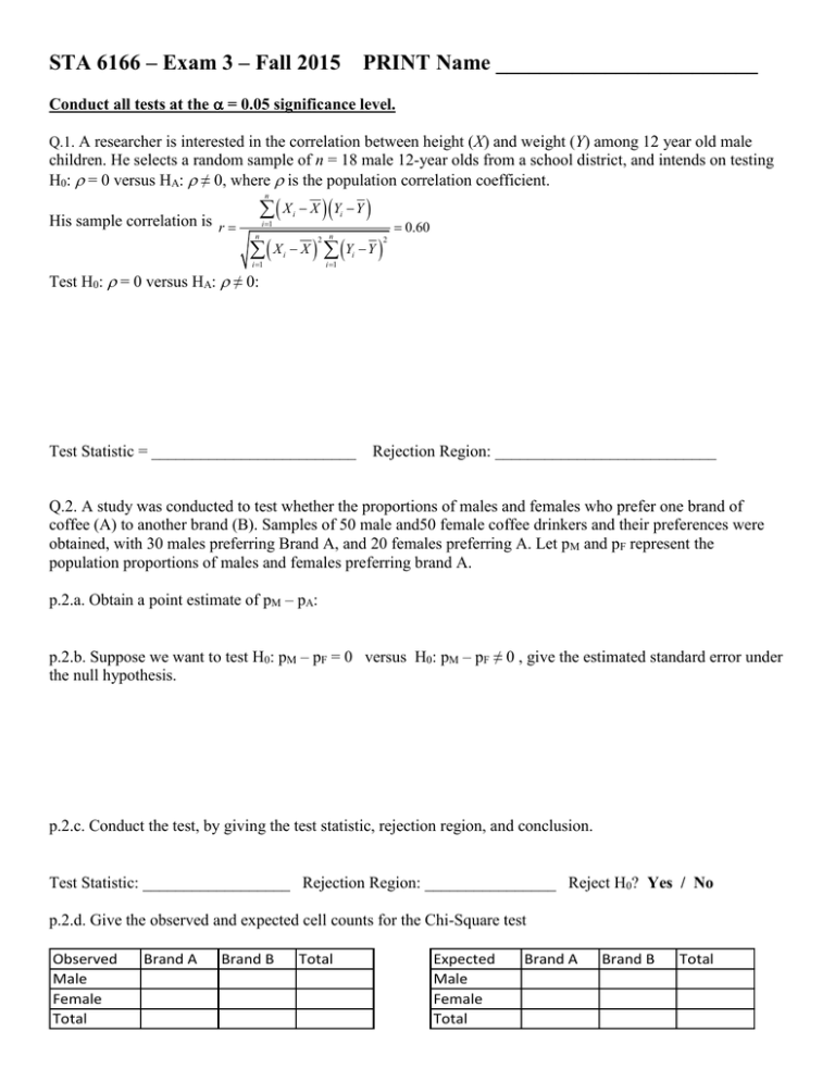
STA 6166 – Exam 3 – Fall 2015
PRINT Name ________________________
Conduct all tests at the  = 0.05 significance level.
Q.1. A researcher is interested in the correlation between height (X) and weight (Y) among 12 year old male
children. He selects a random sample of n = 18 male 12-year olds from a school district, and intends on testing
H0:  = 0 versus HA:  ≠ 0, where  is the population correlation coefficient.
 X
n
His sample correlation is r 
i 1
 X
n
i 1
i
i

 X Yi  Y
X

  Y  Y 
2 n
i 1
 0.60
2
i
Test H0:  = 0 versus HA:  ≠ 0:
Test Statistic = _________________________
Rejection Region: ___________________________
Q.2. A study was conducted to test whether the proportions of males and females who prefer one brand of
coffee (A) to another brand (B). Samples of 50 male and50 female coffee drinkers and their preferences were
obtained, with 30 males preferring Brand A, and 20 females preferring A. Let pM and pF represent the
population proportions of males and females preferring brand A.
p.2.a. Obtain a point estimate of pM – pA:
p.2.b. Suppose we want to test H0: pM – pF = 0 versus H0: pM – pF ≠ 0 , give the estimated standard error under
the null hypothesis.
p.2.c. Conduct the test, by giving the test statistic, rejection region, and conclusion.
Test Statistic: __________________ Rejection Region: ________________ Reject H0? Yes / No
p.2.d. Give the observed and expected cell counts for the Chi-Square test
Observed
Male
Female
Total
Brand A
Brand B
Total
Expected
Male
Female
Total
Brand A
Brand B
Total
Q.3. A company productivity office is interested in the effects of lighting and music on employee productivity.
Factor A (lighting) had 2 levels (soft and bright) and Factor B (music) had 3 levels (jazz, easy listening, and
pop). They selected 30 offices within the firm, and randomly assigned them so that n = 5 received each of the 6
combinations of lighting and music. The response measured was the total output for each office. The summary
data are given below.
Mean Productivity
Lighting\Music Jazz Easy Pop Overall
Soft
30
40
50
40
Bright
20
40
60
40
Overall
25
40
55
40
ANOVA
Source df
Lighting
Music
L*M
Error
Total
SS
MS
5000
48000
57500
F
#N/A
F(0.05)
#N/A
#N/A
p.3.a. Complete the ANOVA table.
p.3.c. Assuming the interaction is not significant, use Bonferroni’s method to compare all 3 pairs of music
types. Which types (if any) are significantly different?
#N/A
#N/A
Q.4. In order to help estimate the peak power demand of a generating plant, data was collected to see if there was a linear
relationship between the forecast high temperature for a day and the peak load demand for that day. Computer analysis of
the data gave the following (abbreviated) results:
Variable
temp
load
Source
Model
Error
Corrected Total
Variable
Intercept
temp
DF
1
1
DF
1
8
9
N
Mean
Std Dev
10
91.400
6.687
10
195.000
45.225
Analysis of Variance
Sum of
Mean
Squares
Square
F Value
16735
16735
80.01
1673
209
18408
Parameter Estimates
Parameter
Standard
Estimate
Error
-394.42097
66.05542
6.44881
0.72097
Pr > F
<.0001
p.4.a. Give a 95% confidence interval for the increase in expected peak load for a 1 degree increase in predicted high
temperature.
p.4.b. Give a point estimate and 95% confidence interval for the mean peak load when the forecast high is 84.
se

1 x * x

n
S xx

2
1  84  91.4 
 14.46

 7.03
10
402.44
2
Point Estimate: __________________________ 95% CI: __________________
p.4.c. Compute r2, the coefficient of determination
Q.5. A regression model is fit, relating height (Y, in cm) to hand length (X1, in cm) and foot length (X2, in cm)
for a sample of n=75 adult females. The following results are obtained from a regression analysis of:
Y = 0 + 1X1 + 2X2 +  ~ NID(0,2)
Regression Statistics
R Square
ANOVA
df
Regression
Residual
Total
Intercept
X1
X2
SS
1105.52
F*
F(0.05)
#N/A
#N/A
#N/A
#N/A
StdErr t*
7.97 #N/A
0.49
0.37
t(.025)
#N/A
1793.85
Coeff
74.41
2.38
1.73
MS
#N/A
#N/A
#N/A
p.5.a. Complete the tables.
p.5.b. The first woman in the sample had a hand length of 19.56cm, a foot length of 25.70cm, and a height of
160.60cm. Obtain her fitted value and residual.
Fitted value = _____________________________________ Residual = _____________________________