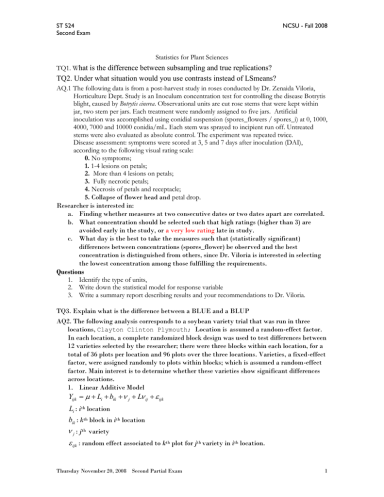
ST 524
Second Exam
NCSU - Fall 2008
Statistics for Plant Sciences
TQ1. What is the difference between subsampling and true replications?
TQ2. Under what situation would you use contrasts instead of LSmeans?
AQ.1 The following data is from a post-harvest study in roses conducted by Dr. Zenaida Viloria,
Horticulture Dept. Study is an Inoculum concentration test for controlling the disease Botrytis
blight, caused by Botrytis cinerea. Observational units are cut rose stems that were kept within
jar, two stem per jars. Each treatment were randomly assigned to five jars. Artificial
inoculation was accomplished using conidial suspension (spores_flowers / spores_i) at 0, 1000,
4000, 7000 and 10000 conidia/mL. Each stem was sprayed to incipient run off. Untreated
stems were also evaluated as absolute control. The experiment was repeated twice.
Disease assessment: symptoms were scored at 3, 5 and 7 days after inoculation (DAI),
according to the following visual rating scale:
0. No symptoms;
1. 1-4 lesions on petals;
2. More than 4 lesions on petals;
3. Fully necrotic petals;
4. Necrosis of petals and receptacle;
5. Collapse of flower head and petal drop.
Researcher is interested in:
a. Finding whether measures at two consecutive dates or two dates apart are correlated.
b. What concentration should be selected such that high ratings (higher than 3) are
avoided early in the study, or a very low rating late in study.
c. What day is the best to take the measures such that (statistically significant)
differences between concentrations (spores_flower) be observed and the best
concentration is distinguished from others, since Dr. Viloria is interested in selecting
the lowest concentration among those fulfilling the requirements.
Questions
1. Identify the type of units,
2. Write down the statistical model for response variable
3. Write a summary report describing results and your recommendations to Dr. Viloria.
TQ3. Explain what is the difference between a BLUE and a BLUP
AQ2. The following analysis corresponds to a soybean variety trial that was run in three
locations, Clayton Clinton Plymouth; Location is assumed a random-effect factor.
In each location, a complete randomized block design was used to test differences between
12 varieties selected by the researcher; there were three blocks within each location, for a
total of 36 plots per location and 96 plots over the three locations. Varieties, a fixed-effect
factor, were assigned randomly to plots within blocks; which is assumed a random-effect
factor. Main interest is to determine whether these varieties show significant differences
across locations.
1. Linear Additive Model
Yijk    Li  bik  j  L ij   ijk
Li : ith location
bik : kth block in ith location
 j : jth variety
 ijk : random effect associated to kth plot for jth variety in ith location.
Thursday November 20, 2008 Second Partial Exam
1
ST 524
Second Exam
NCSU - Fall 2008
2. The estimated mean for jth variety (LSMEANS) may be represented, according the
linear additive model, by,
3   L1  L2  L3   b11  b12  b13  b21  b22  b23  b31  b32  b33 


 j
.
9
9
9
3   L 1 j  L 2 j  L 3 j   1 j1  1 j 2  1 j 3   2 j1   2 j 2   2 j 3   3 j1   3 j 2   3 j 3 


9
9
y. j . 
Y. j .
and its variance is given by
2 2
2
Var y. j .  L   b2( L )  L  e
3
3
9
3. Variance of the difference between variety 1 and 2, on average of all locations,
3   L1  L2  L3   b11  b12  b13  b21  b22  b23  b31  b32  b33 
Y
y.1.  .1.   

 1
9
9
9
3   L 11  L 21  L 31   111  112  113   211   212   213   311   312   313 


9
9
3

L

L

L
b

b

b

b

b
 1 2 3    11 12 13 21 22  b23  b31  b32  b33  
Y
y.2.  .2.   
2
9
9
9
3   L 12  L 22  L 32   121  122  123   221   222   223   321   322   323 


9
9
 
3   L 11  L 21  L 31  3   L 12  L 22  L 32 

9
9
111  112  113   211   212   213   311   312   313  121  122  123   221   222   223   321   322   323 



9
9
  L2  e2 
 L2
 e2
Var y.1.  y.2.  2 
 2
 2 


3
9
9 
 3
y.1.  y.2.   1  2  


4. Estimated mean and variance for variety jth in location ith
y ij . 

Yij .
3


Var y ij . | L 
3   Li 

3
 b2( L )  e2
3

 bi1  bi 2  bi3  
3
j

3   L ij 
3


ij1
  ij 2   ij 3 
3
3
Questions
1. Your advisor has run similar analysis with PROC GLM and wants you to explain whatever
differences are observed in the LSMEANS for Variety 1 and for Location 1.
2. You plan to present the results of the statistical analysis to your research group and need to
explain the differences on the estimated values for Variety 1, and for Location 1.
3. Your advisor has asked you to analyze the Location*Variety interaction, i.e., look at the
Location*Variety means, how would you proceed with the analysis to answer his request?
Thursday November 20, 2008 Second Partial Exam
2
ST 524
Second Exam
NCSU - Fall 2008
Bonus questions
B1. A first-year master student in CALS has asked you for help with the following question.
Please explain concisely your answer to your friend who has limited knowledge of
statistics.
Factors A and B are tested in a factorial design experiment. The levels of each factor and
the response means for each treatment combination are listed:
A
B
Mean
50 10
12
50
2
26
5
10
17
5
2
6
Need to answer the following:
Construct a graph (levels of A on the x-axis, response means on the y-axis) of the means for the
four treatment combinations. Is the A*B interaction significant or not?
B2. Another friend has lost part of the information from a field study conducted before she
started school here and has asked your help in completing the information. Fill in the
missing values.
This is a split plot design in randomized complete blocks. There are 4 blocks which
contain three Pollenizers which were compared on the yield in cucumber. The
investigators are also interest in comparing three Grafts for measuring yield in cucumber.
Within each block, plots were assigned to three pollenizers. Assume blocks to be a random
factor. ANOVA for yield data is presented below:
Source
Blocks
Pollenizers
Main plot error
Grafts
Pollenizers * Grafts
Subplot error
Total
df
3
2
SS
MS
314.2317
6.2637
2
98.3084
10.2606
689.9781
130.2868
24.5771
F
P
150.49
0.0001
228.56
0.0001
1. Your friend says that Grafts is a random effect factor. Present the table of Expected Mean
Squares and show new ANOVA table with corrected F and p values.
2. Write the statistical linear model and hypothesis tested.
3. What conclusions do you draw from this table?
4. What additional statistical analysis would you suggest?
5. Calculate the standard error for a Pollenizers mean on average of Grafts,
6. Calculate the standard error for a Grafts mean on average of Pollenizers,
7. Calculate the standard error for the difference between two interaction (Pollenizers*Grafts)
means, to compare differences in response between two grafts for a common Pollenizer.
8. Calculate the standard error for the difference between two interaction (Pollenizers*Grafts)
means, to compare differences in response between twoPollenizers for a common Grafts.
9. Calculate the standard error for the difference between two interaction (Pollenizers*Grafts)
means, to compare differences in response between two combination means,
Pollenizer_1*Grafts_4 and Pollenizer_3*Graft_2, that are of standard use among farmers.
Thursday November 20, 2008 Second Partial Exam
3