Random Signals for Engineers using MATLAB and Mathcad
Copyright  1999 Springer Verlag NY
Example 6.9 Simulation Linear System with White Noise
In order to develop a simulation of the network we will first change the differential equation to a
difference equation and then excite this discrete circuit with the discrete equivalent of white noise or a
white noise sequence. A white noise process results in the limit when we have a white noise sequence that
has a sample rate approaching infinity. Since we will not be using an infinite sample rate we must adjust
the amplitude of the finite sampled sequence so that the variance of the output of an integrator whose input
is white noise should be the same a white noise sequence input to a discrete summer.
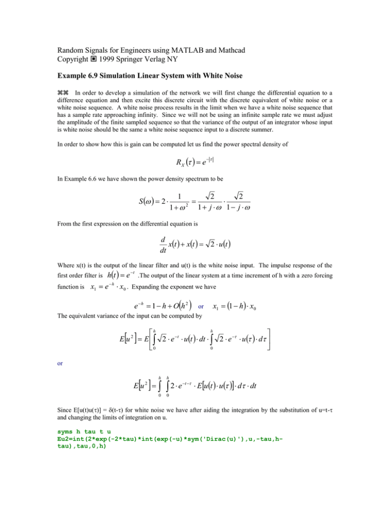
In order to show how this is gain can be computed let us find the power spectral density of
RX    e

In Example 6.6 we have shown the power density spectrum to be
S    2 
1
2
2


2
1  j  1  j 
1
From the first expression on the differential equation is
d
xt   xt   2  u t 
dt
Where x(t) is the output of the linear filter and u(t) is the white noise input. The impulse response of the
ht   e t .The output of the linear system at a time increment of h with a zero forcing
h
function is x1  e  x 0 . Expanding the exponent we have
first order filter is
 
e h  1  h  O h 2
or
x1  1  h   x0
The equivalent variance of the input can be computed by
h
h

E u 2  E   2  e t  u t   dt   2  e   u    d 
0
0

 
or
 
h
Eu 
2
0
h
2e
t 
 Eu t   u    d  dt
0
Since E[u(t)u()] = (t-) for white noise we have after aiding the integration by the substitution of u=t-
and changing the limits of integration on u.
syms h tau t u
Eu2=int(2*exp(-2*tau)*int(exp(-u)*sym('Dirac(u)'),u,-tau,htau),tau,0,h)
Eu2 =
(-1/2-1/2*signum(h))*exp(-2*h)+1/2+1/2*signum(h)
Eu2 =-exp(-2*h)+1
Expanding the exponent we have
taylor(1-exp(-2*h),2)
ans =
2*h
Or the variance of the input white noise sequence should be 2 h and the input white noise sequence should
be scaled by
2 h
Returning to the Example circuit in Example 6.8 we have the difference equation for a discrete
approximation of the differential equation is
y n1  y n
   y n    xn
h
with
R
L
 . Solving for yn+1 we have the difference equation
y n1  1  h     y n  h    xn
where h is the time interval. As discussed, in order to equate the variance of white noise to the white noise
sequence we must compensate for the effective integrator that must be used to obtain a sequence with the
same variance as the continuous system. If the linear system were an integrator and the white noise with the
scale factor of the correlation function amplitude2 is input to an integrator the output is2 t where t is the
time that the integrator is operating. In order to output2 the input variance should be 2/t. As shown
above when the linear system has a time constant we must generate a random white noise sequence of N
points with a normal zero mean density function and a standard deviation of
1
2  h 
to compensate for
the gain change.
Ny=8000;h=0.05;
alp = 0.5;
xstd=1/sqrt(2*h*alp)
x=xstd*randn(Ny,1);
mean(x)
std(x)
xstd =
4.4721
ans =
0.0119
ans =
4.4834
We notice that experimental standard deviation of x is close to the theoretical value of xstd and the mean is
close to zero.
The output sequence is now generated with the following discrete equation
y=zeros(8000,1);
y(1)=0;
for i=1:Ny
y(i+1)=(1-h*alp)*y(i)+h*alp*x(i);
end
mean(y)
std(y)
ans =
0.0074
ans =
0.5098
The result now compares to the theoretical one given below. We have N 0 a values of 4 to make the white
noise spectrum yield a variance of 1 when input to an integrator.
4/4*alp
ans =
0.5000
