Random Signals for Engineers using MATLAB and Mathcad
Copyright  1999 Springer Verlag NY
Example 6.10 Spectrum of White Noise
In the example we will numerically compute the spectrum of a white noise sequence. A white noise
sequence is the discrete equivalent of white noise and processes the property that all the samples are
uncorrelated with each other. When we compute the correlation function and then transform the correlation
function, we expect to obtain a uniform power density function whose amplitude is equal to the variance of
the sequence.
We first generate a uniformly distributed, zero mean sequence and we may compute the mean and variance
of this sequence
N=256
X=rand(N,1)-0.5;
mean(X)
std(X)
N =
256
ans =
-0.0030
ans =
0.2825
and remember that for a uniform distribution we have
Xstd=sqrt(1/12)
Xstd =
0.2887
We
first compute the correlation function by a summation and then take the Fourier transform of this
Xstd=sqrt(1/12)
sequence
Nk=64;
for m=1:Nk
r(m)=1/N*X(1:N-m+1)'*X(m:N);
end
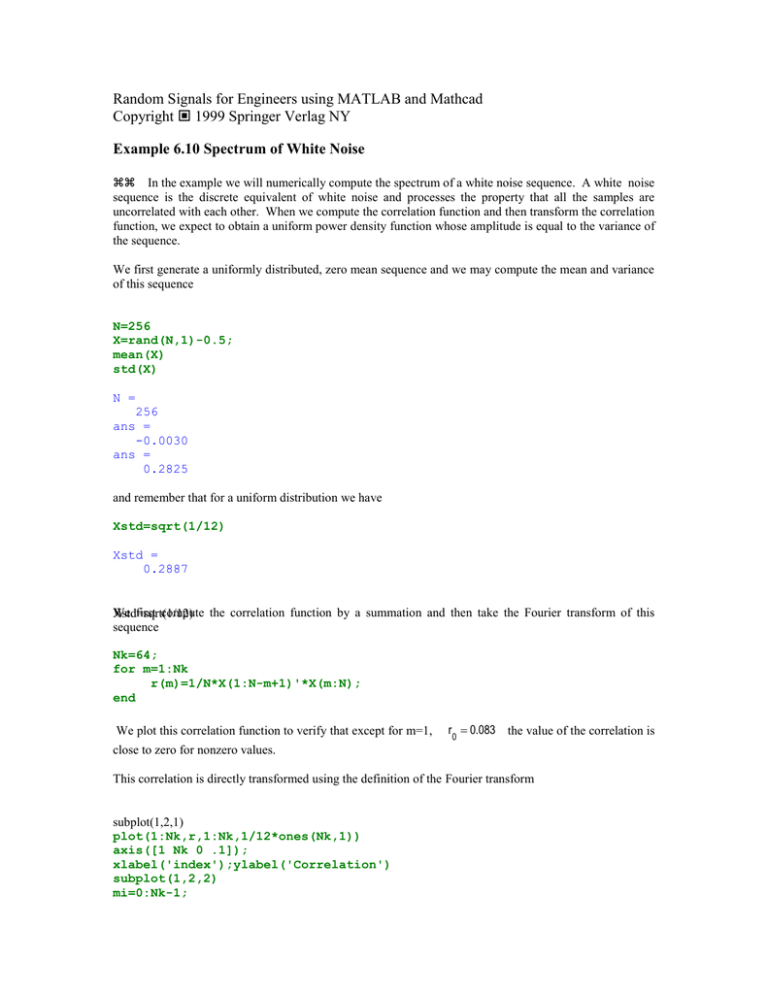
We plot this correlation function to verify that except for m=1,
r0  0.083 the value of the correlation is
close to zero for nonzero values.
This correlation is directly transformed using the definition of the Fourier transform
subplot(1,2,1)
plot(1:Nk,r,1:Nk,1/12*ones(Nk,1))
axis([1 Nk 0 .1]);
xlabel('index');ylabel('Correlation')
subplot(1,2,2)
mi=0:Nk-1;
0.1
0.2
0.09
0.18
0.08
0.16
0.07
0.14
Power Spectrum
Correlation
for m=1:Nk
p(m)=r*exp(-i*(m-1)*pi/Nk*mi)';
end
plot(1:Nk,abs(p),1:Nk,r(1)*ones(Nk,1))
axis([1 Nk 0 .2]);
xlabel('index');ylabel('Power Spectrum')
0.06
0.05
0.04
0.12
0.1
0.08
0.03
0.06
0.02
0.04
0.01
0.02
0
20
40
0
60
20
index
40
60
index
Clearly there are large variations in the computed power spectrum. We now recompute the power spectrum
from the correlation using the built in FFT function. First pad the correlation function with zeros and then
HC=fft(r,2*Nk);
H=abs(HC);
figure
plot(1:Nk,H(1:Nk),'b',1:Nk,abs(p)+.003,'r--',1:Nk,r(1)*ones(1,Nk))
0.16
0.14
0.12
0.1
0.08
0.06
0.04
0
10
20
30
40
50
60
70
We now compute a periodogram directly taking the FFT of the time series and compute the power
spectrum approximation by summing the magnitude of the time series directly and not computing the
correlation function.
G=fft(X,2*Nk);
P=abs(1/2/Nk*G.*conj(G));
plot(1:Nk,P(1:Nk),1:Nk,r(1)*ones(1,Nk))
0.35
0.3
0.25
0.2
0.15
0.1
0.05
0
0
10
20
30
40
50
60
70
Again we find large variations in the power spectrum approximation. The approximation may be improved
by averaging Ns of the points of each periodogram to produce an averaging periodogram each point. The
following summation averages Ns Pi's from kk to kk+Ns-1 for each value of kk. As we average over more
points the variation in the computed periodogram improves. This is shown by computing the periodogram
for Ns= 20 and 60.
for kk=1:Nk
P20(kk) =1/20*sum(P(kk:kk+20-1));
P60(kk) = 1/60*sum(P(kk:kk+60-1));
end
u=1:Nk;
plot(u,P20,u,P60,u,1/12*ones(1,Nk))
0.11
0.1
0.09
0.08
0.07
0.06
0.05
0
10
20
30
40
50
60
70
The graph shows that the uniform value of r0= 0.083 is achieved more closely by averaging 60
periodograms. In order to improve the variations about the constant value we must increase the size of the
data and perform more averaging.
