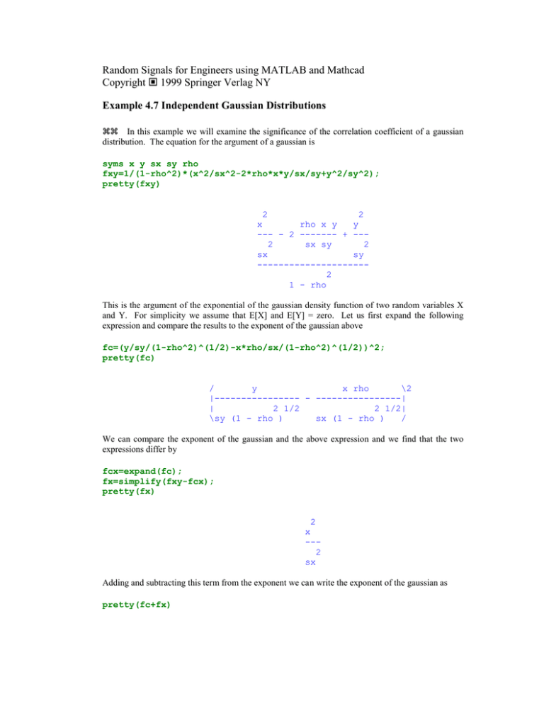
Random Signals for Engineers using MATLAB and Mathcad
Copyright  1999 Springer Verlag NY
Example 4.7 Independent Gaussian Distributions
In this example we will examine the significance of the correlation coefficient of a gaussian
distribution. The equation for the argument of a gaussian is
syms x y sx sy rho
fxy=1/(1-rho^2)*(x^2/sx^2-2*rho*x*y/sx/sy+y^2/sy^2);
pretty(fxy)
2
2
x
rho x y
y
--- - 2 ------- + --2
sx sy
2
sx
sy
--------------------2
1 - rho
This is the argument of the exponential of the gaussian density function of two random variables X
and Y. For simplicity we assume that E[X] and E[Y] = zero. Let us first expand the following
expression and compare the results to the exponent of the gaussian above
fc=(y/sy/(1-rho^2)^(1/2)-x*rho/sx/(1-rho^2)^(1/2))^2;
pretty(fc)
/
y
x rho
\2
|---------------- - ----------------|
|
2 1/2
2 1/2|
\sy (1 - rho )
sx (1 - rho )
/
We can compare the exponent of the gaussian and the above expression and we find that the two
expressions differ by
fcx=expand(fc);
fx=simplify(fxy-fcx);
pretty(fx)
2
x
--2
sx
Adding and subtracting this term from the exponent we can write the exponent of the gaussian as
pretty(fc+fx)
2
/
y
x rho
\2
x
|---------------- - ----------------| + --|
2 1/2
2 1/2|
2
\sy (1 - rho )
sx (1 - rho )
/
sx
We now compute the conditioned gaussian density function or
f ( y| X  x ) 
f ( x, y)
f ( x)
The expanded exponent can be used to simplify the computation of the numerator and denominator
of the density function by performing the following transformation from z=f(xy) and w=x
pretty( [y/sy/(1-rho^2)^(1/2)-x*rho/sx/(1-rho^2)^(1/2); x ])
[
y
x rho
]
[---------------- - ----------------]
[
2 1/2
2 1/2]
[sy (1 - rho )
sx (1 - rho )
]
[
]
[
x
]
The Jacobian of this transformation is
jac=jacobian([y/sy/(1-rho^2)^(1/2)-x*rho/sx/(1-rho^2)^(1/2);x],[x
y])
djac=det(jac)
jac =
[ -rho/sx/(1-rho^2)^(1/2),
[
1,
djac =
-1/sy/(1-rho^2)^(1/2)
1/sy/(1-rho^2)^(1/2)]
0]
syms z w
z= y/sy/(1-rho^2)^(1/2)-x*rho/sx/(1-rho^2)^(1/2)
z =
y/sy/(1-rho^2)^(1/2)-x*rho/sx/(1-rho^2)^(1/2)
The marginal density function is found by integrating over z or
f  x   f w  

 f z, w  dz


f ( z , w) 
e
1 w2
2  x2
2 x y 1  
f ( w) 

1
2 x
e
2
e
1 w2
2  x2
1 z 2
2


e

z2
2

y
1  2

dz
2 
The integral in z is just a normal gaussian and equal to
Since f(w) is just f(x) we have
f ( x) 

1
e
2   x
1 x2
2  x2
The numerator has already been expanded in terms of z and the denominator just cancels the f(x)
term to obtain
f ( y X  x) 
1
2   y

1
exp 
2
 2  1   2   y2
1 



2

 

x
 y   
 x 

 

y

 
For simplicity we have assumed the x and y have zero means. If we were to replace the means in the
above expression by substitution of x = x' - ax and y = y' - ay and then dropping the prime, the
resultant expression now contains the means. We recognize that the conditional expression is just a
gaussian density function in y with the mean
ay   
x
 x  a x 
y
and a variance of
1    
2
The expected value of this expression is
EY X  x  a y   
2
y
x
 x  a x 
y
It is easy to show that the COV[X Y ] = x y by multiplying the density function by x / x and
y /y and changing variables to z and w and performing the integration.
The above expression can be used to show the independence of the two gaussian variables X and Y.
When X and Y are uncorrelated or the COV[X Y] = 0 then  = 0. The expected value of y, given that
we know X=x, is just the expected value of y plus  scaled by the ratio of the variances of y and x
time x - ax. This means that y is a linear function of x.
It is interesting to take the limit of the conditional density function as  ± 1. The variance about
the conditional mean approaches zero and the conditional density function of y approaches a delta
function at the conditional mean. This says that y approaches the conditional mean with probability
one.
A matrix can be used to express the variance and covariance of the joint random variables X and Y.
This matrix representation is useful for multiple random variables. We express the covariance
matrix, K as
K=[sx^2 rho*sx*sy ; rho*sx*sy sy^2]
K =
[
sx^2, rho*sx*sy]
[ rho*sx*sy,
sy^2]
Matlab can be used to invert the matrix K.
pretty(K^(-1))
[
1
[- --------------[
2
2
[ sx (-1 + rho )
[
[
rho
[----------------[
2
[sx sy (-1 + rho )
rho
]
-----------------]
2 ]
sx sy (-1 + rho )]
]
1
]
- ---------------]
2
2 ]
sy (-1 + rho )]
The determinant can also be computed as
det(K)
ans =
sx^2*sy^2-rho^2*sx^2*sy^2
We notice by direct multiplication that the matrix expression
E=[x y]*K^(-1)*[x y].';
pretty(simplify(E))
2
2
2
2
x sy - 2 x sy y rho sx + y sx
- --------------------------------2
2
2
sx sy (-1 + rho )
The last expression is just the exponent of the gaussian density function and we may write the
gaussian density in matrix form as
f  x, y  
 1
 exp    x
2   K
 2
1
 x 
y   K 1   
 y 
