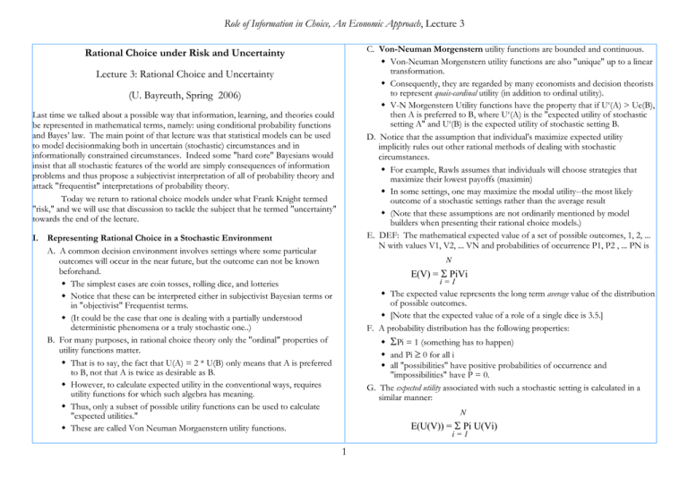
Role of Information in Choice, An Economic Approach, Lecture 3
C. Von-Neuman Morgenstern utility functions are bounded and continuous.
Von-Neuman Morgenstern utility functions are also "unique" up to a linear
transformation.
Consequently, they are regarded by many economists and decision theorists
to represent quais-cardinal utility (in addition to ordinal utility).
V-N Morgenstern Utility functions have the property that if Ue(A) > Ue(B),
then A is preferred to B, where Ue(A) is the "expected utility of stochastic
setting A" and Ue(B) is the expected utility of stochastic setting B.
D. Notice that the assumption that individual's maximize expected utility
implicitly rules out other rational methods of dealing with stochastic
circumstances.
For example, Rawls assumes that individuals will choose strategies that
maximize their lowest payoffs (maximin)
In some settings, one may maximize the modal utility--the most likely
outcome of a stochastic settings rather than the average result
(Note that these assumptions are not ordinarily mentioned by model
builders when presenting their rational choice models.)
E. DEF: The mathematical expected value of a set of possible outcomes, 1, 2, ...
N with values V1, V2, ... VN and probabilities of occurrence P1, P2 , ... PN is
Rational Choice under Risk and Uncertainty
Lecture 3: Rational Choice and Uncertainty
(U. Bayreuth, Spring 2006)
Last time we talked about a possible way that information, learning, and theories could
be represented in mathematical terms, namely: using conditional probability functions
and Bayes’ law. The main point of that lecture was that statistical models can be used
to model decisionmaking both in uncertain (stochastic) circumstances and in
informationally constrained circumstances. Indeed some "hard core" Bayesians would
insist that all stochastic features of the world are simply consequences of information
problems and thus propose a subjectivist interpretation of all of probability theory and
attack "frequentist" interpretations of probability theory.
Today we return to rational choice models under what Frank Knight termed
"risk," and we will use that discussion to tackle the subject that he termed "uncertainty"
towards the end of the lecture.
I. Representing Rational Choice in a Stochastic Environment
A. A common decision environment involves settings where some particular
outcomes will occur in the near future, but the outcome can not be known
beforehand.
The simplest cases are coin tosses, rolling dice, and lotteries
Notice that these can be interpreted either in subjectivist Bayesian terms or
in "objectivist" Frequentist terms.
(It could be the case that one is dealing with a partially understood
deterministic phenomena or a truly stochastic one..)
B. For many purposes, in rational choice theory only the "ordinal" properties of
utility functions matter.
That is to say, the fact that U(A) = 2 * U(B) only means that A is preferred
to B, not that A is twice as desirable as B.
However, to calculate expected utility in the conventional ways, requires
utility functions for which such algebra has meaning.
Thus, only a subset of possible utility functions can be used to calculate
"expected utilities."
These are called Von Neuman Morgaenstern utility functions.
N
E(V) = Σ PiVi
i=1
The expected value represents the long term average value of the distribution
of possible outcomes.
[Note that the expected value of a role of a single dice is 3.5.]
F. A probability distribution has the following properties:
ΣPi = 1 (something has to happen)
and Pi ≥ 0 for all i
all "possibilities" have positive probabilities of occurrence and
"impossibilities" have P = 0.
G. The expected utility associated with such a stochastic setting is calculated in a
similar manner:
N
E(U(V)) = Σ Pi U(Vi)
i=1
1
Role of Information in Choice, An Economic Approach, Lecture 3
where the value of the possible outcomes is now measured in utility terms.
E(U(V)) is more commonly written as Ue(V)
H. Ue(V) is not generally equal to U(Ve).
Ue(V) is the same as U(Ve) only if U is a linear function.
In such cases, the individual is said to be risk neutral.
(In effect this method of calculating an individual's demand for information
requires calculating an expected value of an expected value, insofar as one
also has to estimate the information that will be obtained.)
E. Of course, the value of certain information (facts) to an individual depends
partially on the choice setting.
Knowing the value of the next roll of the dice or turn of the roulette table,
could be worth enormous sums of money!
Knowing the size of one's foot to three decimal places may be worth next
to nothing, because no decision can be improved by knowing that
information.
II. DEF: An individual is said to be risk averse if the expected utility of some
gamble or risk is less than the utility generated at the expected value
(mean) of the variable being evaluated.
A risk neutral individual is one for whom the expected utility of a gamble
(risky situation) and utility of the expected (mean) outcome are the same.
A risk preferring individual is one for whom the expected utility of a gamble
is greater than the utility of the expected (mean) outcome.
The more risk averse a person is, the greater is the amount that he or she is
willing to pay to avoid a risk.
A. Note that this implies that any utility function that is strictly concave with
respect to income, exhibits risk aversion. (Why?)
[depict expected utility on a diagram, note risk premium, etc.]
B. More formally, the degree of risk aversion can be measured using the
Arrow-Pratt measure of (absolute) risk aversion:
r(Y) = - U"(Y)/U'(Y)
C. Discrete expected utility maximizing models are relatively easy to manipulate
and are widely used to model the demand for insurance, the demand for
information, and to characterize both mixed strategies and mixed strategy
equilibria.
D. The demand for information can be represented in several ways in these
"discrete event spaces."
For example, both Bayesian (statistical) and Shannon (communcation
theory) measures of information assume that uncertainty tends to fall as
individuals become better informed.
Thus, information or this sort makes individuals better off by increasing
certatainty.
The amount that an individual would be willing to pay for information that
is conclusive (e.g. produces complete certainty) is approximately equal to
his her or risk premium in the setting of interest.
III. Models of expected utility maximizing decisionmaking can also be
constructed for "continuous event spaces" by using probability density
functions that map over intervals or real number lines to represent event
spaces.
A. These representations are widely used in economic analysis and in
econometrics and decision making (and learning) under uncertainty where the
event space is continuous (i. e., convex).
For example, it is often convenient to represent uncertainty with a uniform
distribution distributed between some Low and High values.
These are mathematically very easy to manipulate.
The normal distribution is also used, especially in statistical work, because
it is thought to characterize a broad range of real-world probability
distributions--although it is mathematically very inconvenient to manipulate.
B. A continuous probability distribution, by definition, has properties that are
very similar to those of the discrete distributions looked discussed above.
The "sum" of the "probabilities" again equals 1.
Let f(x) be a density function, then
+∞
∫ f(x)dx = 1
−∞
(Areas under the density function are probabilities, and they must add up to
one--"something" has to happen..)
Again, no value of the density function can be less than zero, f(x) > 0, for
all x.
An event can not have a negative probability of occurrence!
C. Expected value again represents the large sample average value of the
distribution of outcomes.
2
Role of Information in Choice, An Economic Approach, Lecture 3
+∞
profit will bring into relief the nature of the distinction between the perfect
competition of theory and the remote approach which is made to it by the actual
competition of, say, twentieth-century United States; and the answer to this twofold
problem is to be found in a thorough examination and criticism of the concept of
Uncertainty, and its bearings upon economic processes.
I.I.25
But Uncertainty must be taken in a sense radically distinct from the familiar notion of
Risk, from which it has never been properly separated. The term "risk," as loosely used
in everyday speech and in economic discussion, really covers two things which,
functionally at least, in their causal relations to the phenomena of economic
organization, are categorically different. The nature of this confusion will be dealt with
at length in chapter VII, but the essence of it may be stated in a few words at this
point. The essential fact is that "risk" means in some cases a quantity susceptible of
measurement, while at other times it is something distinctly not of this character; and
there are far-reaching and crucial differences in the bearings of the phenomenon
depending on which of the two is really present and operating. There are other
ambiguities in the term "risk" as well, which will be pointed out; but this is the most
important. It will appear that a measurable uncertainty, or "risk" proper, as we shall use
the term, is so far different from an unmeasurable one that it is not in effect an
uncertainty at all. We shall accordingly restrict the term "uncertainty" to cases of the
non-quantitive type. It is this "true" uncertainty, and not risk, as has been argued,
which forms the basis of a valid theory of profit and accounts for the divergence
between actual and theoretical competition.”
E(x) = ∫ v(x)f(x)dx
−∞
D. The expected utility of such a setting is calculated in a similar manner:, but the
"value" of possible outcomes is measured in utility terms.
+∞
E(U(x)) = ∫ U(x)f(x)dx
−∞
E. For example, suppose that utility is U = Yn and it is known that Y (income) is
uniformly distributed between 50 and 150. In this case, f(x) = 0 for x< 50 and
x> 150 so expected utility is:
150
E(U(x)) = ∫
50
1
Y n dY
100
=
(150) n+1 −(50) n+1
100(n+1)
This can be evaluated in the case where n is known. For example, if n = 1,
E(U) =and f(x) = 1/100 for 50< x < 150. (Why?) Expected utility is: 100.
IV. Risk, Uncertainty, and Profit (1921)
An Excerpt from the Introduction:
“As the title of the essay indicates, our task will be envisaged from the immediate
standpoint of the problem of profit in distributive theory. The primary attribute of
competition, universally recognized and evident at a glance, is the "tendency" to
eliminate profit*12 or loss, and bring the value of economic goods to equality with
their cost. Or, since costs are in the large identical with the distributive shares other
than profit, we may express the same principle by saying that the tendency is toward a
remainderless distribution of products among the agencies contributing to their
production. But in actual society, cost and value only "tend" to equality; it is only by an
occasional accident that they are precisely equal in fact; they are usually separated by a
margin of "profit," positive or negative. Hence the problem of profit is one way of
looking at the problem of the contrast between perfect competition and actual
competition.
I.I.24
Our preliminary examination of the problem of profit will show, however, that the
difficulties in this field have arisen from a confusion of ideas which goes deep down
into the foundations of our thinking. The key to the whole tangle will be found to lie in
the notion of risk or uncertainty and the ambiguities concealed therein. It is around this
idea, therefore, that our main argument will finally center. A satisfactory explanation of
A. Frank Knights famous dissertation written in 1921, was one of the first
systematic efforts to understand how what he termed "risk and uncertainty"
affects economic activity.
Although the book is quite old, it is one of the very best statements of the
logic of perfectly competitive markets that have ever been written.
And, it does an excellent job of thinking through the implications of various
kinds of stochastic environments.
B. Knight stresses the difference between what he calls "risky" environments and
"uncertain" environments.
Although his specific terminology did not permanently "catch on" in
economics, his ideas did.
In Knight’s words: “It will appear that a measurable uncertainty, or "risk"
proper, as we shall use the term, is so far different from an unmeasurable
3
Role of Information in Choice, An Economic Approach, Lecture 3
one that it is not in effect an uncertainty at all. We shall accordingly restrict
the term "uncertainty" to cases of the non-quantitive type.”
That is to say, there are differences between what he calls “risk,”
measurable uncertainty--cases in which the probability function is or can
be known, and truly uncertain cases in which the probability function is
not or cannot be know (unmeasurable uncertainty).
C. In a setting in which the probability function can be known, it is possible to
pool risk, and by the law of large numbers (samples) reduce its effect to trivial
levels.
Thus, an insurance company that has millions of companies, in effect, has
an infinite sample and the expected result is more or less the actual result.
In such cases, competition will (or at least can) diminish rates of return to
those of comparable industries.
Here, the expected value calculations used above, truly are expected values
because the sampling error is very small in large samples.
(The standard error of a sample mean is the standard deviation of the
parent distribution divided by the square root of N, the sample size, thus in
the limit the standard error approaches zero.)
D. However, he argues that in circumstances in which “ the probability function”
can not be known (or samples are small) the risk associated with uncertainty
remains.
It is from choices in such environments that profits and losses emerge in a
perfectly competitive market.
Because of unavoidable variance in the outcomes, some person win and
other lose.
(Knight terms such “risk takers” entrepreneurs. They are the persons who
make investments based on their faith or confidence rather than careful
calculations--because careful calculations cannot be made in such
circumstances.)
E. Knight’s relevance for this course, is that he is one of the first to point out
clearly that what can and cannot be known at a given time, can have clear
economic effects--even in an otherwise perfectly competitive model.
(Many textbook treatments of perfect competition simply ignore the
problem by assuming perfect information.)
F.
4