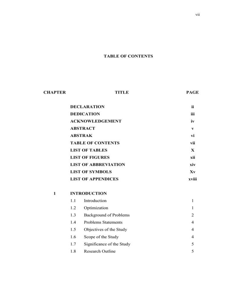
vii
TABLE OF CONTENTS
CHAPTER
TITLE
DECLARATION
ii
DEDICATION
iii
ACKNOWLEDGEMENT
iv
ABSTRACT
v
ABSTRAK
vi
TABLE OF CONTENTS
vii
LIST OF TABLES
X
LIST OF FIGURES
xii
LIST OF ABBREVIATION
xiv
LIST OF SYMBOLS
Xv
LIST OF APPENDICES
1
PAGE
xviii
INTRODUCTION
1.1
Introduction
1
1.2
Optimization
1
1.3
Background of Problems
2
1.4
Problems Statements
4
1.5
Objectives of the Study
4
1.6
Scope of the Study
4
1.7
Significance of the Study
5
1.8
Research Outline
5
viii
2
3
LITERATURE REVIEW
2.1
Introduction
7
2.2
Global Optimization Methods
8
2.3
Global Optimization
9
2.4
Homotopy
10
2.5
Intermediate Value Theorem
13
2.6
Predictor-Corrector Halley Method
14
2.7
Complexity Analysis
16
2.8
Mathematica 8.0
18
2.9
Summary
21
RESEARCH METHODOLOGY
3.1
Introduction
22
3.2
Research Design and Procedure
23
3.3
Homotopy
28
3.3.1 Homotopy Continuation Method (HCM)
28
3.3.2 Homotopy Optimization Method (HOM)
32
3.3.3 Homotopy Optimization with
33
Perturbations and Ensembles method
(HOPE)
3.4
Intermediate Value Theorem (IVT)
34
3.5
Predictor-Corrector Halley's Method (PCH)
39
3.6
Homotopy 2-Step Predictor-corrector Method
40
(HSPM)
3.7
4
Complexity Analysis
44
3.7.1 Time Complexity Analysis (TCA)
44
3.7.2 Space Complexity Analysis (SCA)
45
RESULT AND DISCUSSION
4.1
Introduction
50
4.2
Test Problems
50
ix
4.2.1 Ability to Locate Local Minimizer
51
4.2.2 Ability to Locate More Than One Global
56
Solution
4.2.3 Ability of HSPM Over HOPE
59
Numerical Computation
63
4.3.1 Wilkinson Function
64
4.3.2 Dixon Function
67
4.3.3 Michalewicz Function
69
4.3.4 Dixon-Szego Function
72
4.3.5 Goldstein-Price Function
77
4.3.6 Summary
79
4.4
A Comparison of Success Rate
79
4.5
Complexity Analysis
88
4.5.1 Time Complexity Analysis (TCA)
89
4.5.2 Space Complexity Analysis (SCA)
95
4.5
Comparison between HOPE and HSPM
98
4.6
Conclusion
100
4.3
5
SUMMARY AND CONCLUSION
5.1
Summary of Study
101
5.2
Conclusion
103
5.3
Suggestions for Future Work
103
REFERENCES
105
Appendices A-D
108-123
x
LIST OF TABLES
TABLE NO.
2.1
TITLE
PAGE
Comparison advantages of Mathematica and
other systems in automation.
2.2
Comparison advantages of Mathematica and
other systems in integrated all-in-one platform.
2.3
19
19
Comparison advantages of Mathematica and
other
systems
in
hybrid
symbolic-numeric
20
methodology.
2.4
Comparison advantages of Mathematica and
other systems in multiparadigm language.
3.1
Limit on problem size as determined by growth
rate.
20
47
3.2
Tenfold increase in speed.
48
4.1
Functions used for testing the strengths of HSPM.
51
4.2
Numerical result of Wilkinson function.
65
4.3
Numerical result of Dixon function.
69
4.4
Numerical result of Michalewicz function using
Newton's method.
4.5
Numerical result of Michalewicz function using
HSPM..
4.6
Numerical
result
of
Dixon-Szego
function
computed with good parameter s.
4.7
Numerical
result
of
Dixon-Szego
computed with poor parameter s.
function
71
72
75
76
xi
4.8
Numerical result of Goldstein-Price function.
4.9
Computation of value m according to the
parameter k and N.
4.10
Numerical result of 10-modal Sine function when
m2.
4.11
Success rate of HOPE and HSPM when N=10.
4.12
Computing the worst case time complexity of
HOPE.
4.13
Computing the worst case time complexity of
HSPM.
4.14
Computing the best case time complexity of
HOPE.
4.15
Computing the best case time complexity of
HSPM.
4.16
Time complexity of HOPE and HSPM.
4.17
Computing function HOPE(x) and HSPM(x)
when x=2, 20, 200.
4.18
Space complexity of HOPE in best and worst
case.
4.19
Space complexity of HSPM in best and worst
case.
4.20
Space complexity of HOPE and HSPM.
4.21
Time and space complexities of HOPE and
HSPM (worst case).
4.22
Comparison of HOPE and HSPM
77
80
83
85
90
91
91
92
93
93
96
97
98
98
100
xii
LIST OF FIGURES
FIGURE NO.
TITLE
PAGE
3.1
Operational framework of the research.
25
3.2
Local minimum and global minimum.
26
3.3
Intermediate value theorem.
35
3.4
Flow chart of algorithm HSPM.
43
4.1
Wilkinson function.
52
4.2
Dixon function.
54
4.3
Michalewicz function.
55
4.4
Dixon-Szego function.
57
4.5
Goldstein-Price function.
59
4.6
N-modal Sine Function and its correspond
61
auxiliary functions with
N  10, 20,30, 40,50,60 respectively.
4.7
Wilkinson Function varies from   0 to   1 .
64
4.8
Value of H '( x,0.6) based on s  0.01 and
67
s  0.001 .
4.9
Dixon Function varies from   0 to   1 .
68
4.10
Michalewicz Function varies from   0 to
70
  1.
4.11
Dixon-Szego Function varies from   0 to
73
  1.
4.12
Derivative values of Dixon-Szego function for
s  0.2 and 0.3 re+spectively.
74
xiii
4.13
Goldstein-Price Function varies from   0 to
77
  1.
4.14
10-modal Sine function varies from   0 to
81
  1.
4.15
Result of success rate (%) of HOPE (Dunlavy,
85
2005) and HSPM for N=10.
4.16
Result of success rate (%) of HOPE (Dunlavy,
86
2005) and HSPM for N=20, 30, 40, 50, and 60
respectively.
4.17
Growth rates for n3 and n5 with input size
94
n  5.
4.18
Growth rates for n3 and n5 with input size
n  100 .
94
xiv
LIST OF ABBREVIATIONS
DAEs
-
Differential Algebraic Equations
GO
-
Global Optimization
GOM
-
Global Optimization Methods
HR
-
Hit and Run method
HOPE
-
Homotopy Optimization with Perturbations and
Ensembles
HAM
-
Homotopy Analysis Method
HCM
-
Homotopy Continuation Method
HOM
-
Homotopy Optimization Method
HPM
-
Homotopy Perturbation Method
HSPM
-
Homotopy 2-Step Predictor-corrector Method
IVT
-
Intermediate Value Theorem
M8
-
Mathematica version 8.0
min
-
Minimize/ minimum
max
-
Maximize/ maximum
ODEs
-
Ordinary Differential Equations
PCH
-
Predictor-Corrector Halley's method
sup
-
Supremum
SCA
-
Space Complexity Analysis
TCA
-
Time Complexity Analysis
xv
LIST OF SYMBOLS

-
A closed set which contained solution, big-Omega
notation
K
-
A corresponding value of c over function f, constant
HOPE ( x) ,
-
A function
D
-
A nonempty, closed set
c
-
A value/ element in between interval [a, b]
g ( x)
-
Auxiliary function
O
-
Big oh notation, constant

-
Big theta notation
L,P
-
Constant
k
-
Constant, number of iteration
m
-
Controller of the sharpness of valley of Eq (4.7),
HSPM ( x)
parameter to adjust the step size st
h
-
Convergence-control parameter
ci , i  1, 2,...
-
Cost used for an algorithm
▄
-
End of proof
x*
-
Extremizers
f ( x)
-
Function f or target function
x (1)
-
Global solution
H ( x,  )
-
Homotopy function

-
Homotopy parameter
subintervali
-
i number of subintervals within interval [a, b]
xvi

-
Infinitesimal change of the dependent variable, error,
stopping criterion

-
Infinitesimal increment of the independent variable
In
-
Interval
x 0 , x0
-
Initial guess
xi ,0
-
Initial point, randomly select from subintervali
x (jk 1)
-

-
Least upper bound for A
a
-
Lower bound of an interval
an
-
Lower bound of interval I n
ai
-
Lower bound of subintervali
cmax
-
Maximum number of points in an ensemble
M
-
Maximum number of subintervali , constant
mpt
-
Midpoint of interval
d
-
Non-empty subset of
n, j, i
-
Number of iteration
c
-
Number of perturbations generated of each point in the
j th point in the ensemble at the start of iteration k
ensemble
c ( k 1)
-
Number of points in the ensemble at the beginning of
iteration k
-ve
-
Negative value
F ( x)
-
Objective function

-
Perturbation
x (jk,0)
-
( k 1)
Point found by minimization starting at x j
x (jk,i)
-
Point found by minimization starting at the ith
( k 1)
perturbation of x j
+ve
-
Positive value
X, Y
-
Set
O( g (n)),
-
Set of complexity function
O(h(n)) ,
xvii
A
-
Set contaning element lower bound of I n
n
-
Size input, number of iteration, constant
-
Step length/ step size
xk
-
Solution computed by local search
SBHOPE (n)
-
Space complexity of HOPE in best case
SWHOPE (n)
-
Space complexity of HOPE in worst case
SBHSPM (n)
-
Space complexity of HSPM in best case
SWHSPM (n)
-
Space complexity of HSPM in worst case
c3
-
Three-times-continuously differentiable
TWHOPE (n)
-
Time complexity of HOPE in worst case
TBHOPE (n)
-
Time complexity of HOPE in best case
TWHSPM (n)
-
Time complexity of HSPM in worst case
TBHSPM (n)
-
Time complexity of HSPM in best case
c2
-
Twice-continuously differentiable
b
-
Upper bound of an interval
bn
-
Upper bound of interval I n
bi
-
Upper bound of subintervali
x
-
Variable
 (k )
-
Value of parameter homotopy in iteration k
 , (k ) ,  ,
s , st
xviii
LIST OF APPENDICES
APPENDIX
A
TITLE
Numerical Results for another Four
PAGE
108
Experiments of 10-modal Sine Function
B
HSPM Programming Coded by Mathematica
119
C
Newton's Method (Optimization Version)
122
Programming Coded by Mathematica
D
List of Publication
123