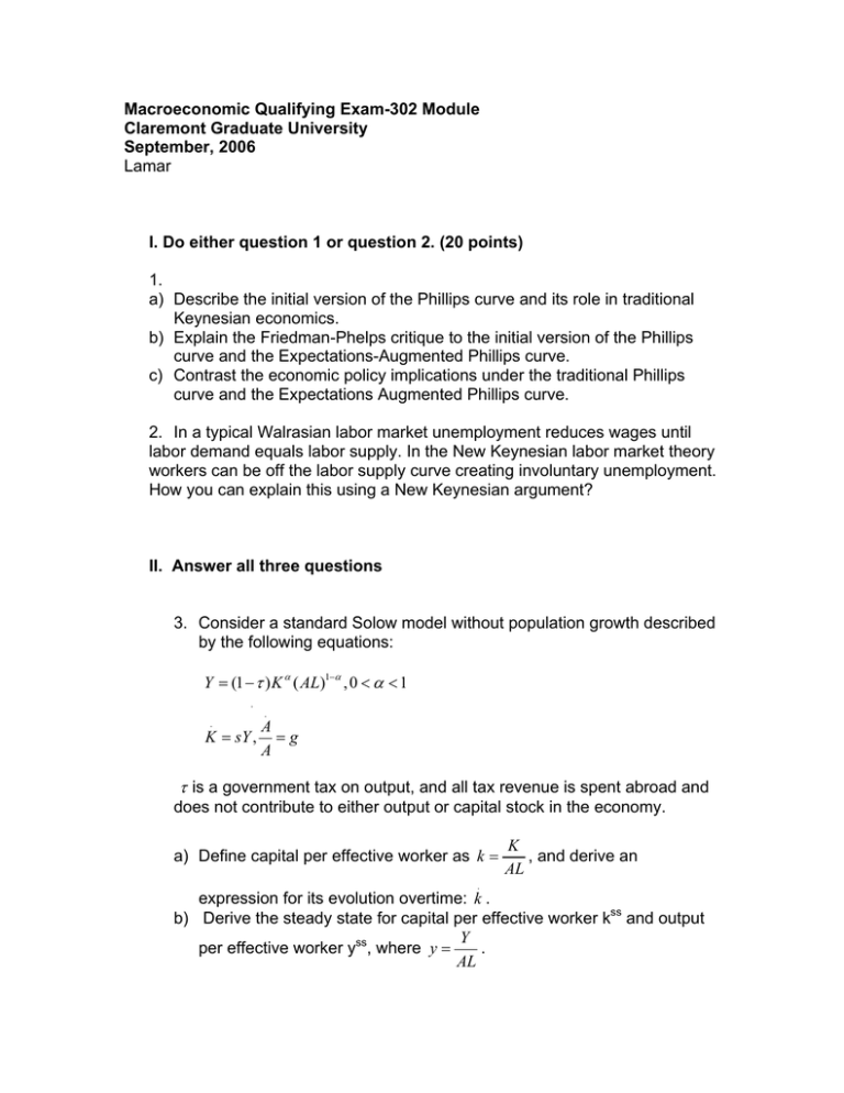
Macroeconomic Qualifying Exam-302 Module
Claremont Graduate University
September, 2006
Lamar
I. Do either question 1 or question 2. (20 points)
1.
a) Describe the initial version of the Phillips curve and its role in traditional
Keynesian economics.
b) Explain the Friedman-Phelps critique to the initial version of the Phillips
curve and the Expectations-Augmented Phillips curve.
c) Contrast the economic policy implications under the traditional Phillips
curve and the Expectations Augmented Phillips curve.
2. In a typical Walrasian labor market unemployment reduces wages until
labor demand equals labor supply. In the New Keynesian labor market theory
workers can be off the labor supply curve creating involuntary unemployment.
How you can explain this using a New Keynesian argument?
II. Answer all three questions
3. Consider a standard Solow model without population growth described
by the following equations:
Y = (1 − τ ) K α ( AL)1−α , 0 < α < 1
.
.
A
K = sY , = g
A
.
τ is a government tax on output, and all tax revenue is spent abroad and
does not contribute to either output or capital stock in the economy.
a) Define capital per effective worker as k =
K
, and derive an
AL
.
expression for its evolution overtime: k .
b) Derive the steady state for capital per effective worker kss and output
Y
per effective worker yss, where y =
.
AL
c) What would be the effect of an increase in the tax rate on actual
investment in the economy and the steady state of output per effective
worker ?
d) Now assume that the tax on output also hurts individual’s incentives to
invent new technologies. Specifically assume that the growth rate of
1
technology, g, is given by g = b(1 − τ ) α where b>0. What is the new
steady state level of output per effective worker? What is the effect of
an increase in the tax on yss now?
e) Explain in words, or graphically, the result you got in d).
(30 points)
4. Consider a simple IS-LM model.
a) Graphically derive the Aggregate Demand curve.
Now assume that total expenditure is given by E (Y , i − Π e , G, T )
where 0 < EY < 1, Ei −Πe < 0, EG = 1, ET < 0. Also assume real money
demand equals L(i, Y ) where Li < 0 LY > 0 .
b) Show graphically what is the effect on output of an increase in
G. What assumption is important in order to explain this result?
What happens to the Aggregate Demand curve?
c) Show algebraically the effect on output of an increase in G.
d) When the crowding-out effect is insignificant?
(30 points)
−
5. Consider a labor market with flexible wages but prices fixed at P = P .
Assume an upward sloping labor supply curve, and assume firms will
meet demand at the prevailing price as long as it does not exceed the
level where marginal cost equals price; denote this level of output by
YMAX.
a) Show the labor market equilibrium of this model in ((W/P),L)
space. Be sure to label the curves, equilibrium labor and wages.
b) Does this model explain involuntary unemployment? Why?
c) How will real wages, employment, and output respond to a
negative aggregate demand shock in this model? Please show
this graphically. Given your results, describe the effect of a
contractionary monetary policy on income, the real wage, and
unemployment in this economy.
(20 points)