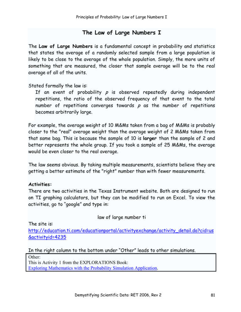
Principles of Probability: Law of Large Numbers I
The Law of Large Numbers I
The Law of Large Numbers is a fundamental concept in probability and statistics
that states the average of a randomly selected sample from a large population is
likely to be close to the average of the whole population. Simply, the more units of
something that are measured, the closer that sample average will be to the real
average of all of the units.
Stated formally the law is:
If an event of probability p is observed repeatedly during independent
repetitions, the ratio of the observed frequency of that event to the total
number of repetitions converges towards p as the number of repetitions
becomes arbitrarily large.
For example, the average weight of 10 M&Ms taken from a bag of M&Ms is probably
closer to the "real" average weight than the average weight of 2 M&Ms taken from
that same bag. This is because the sample of 10 is larger than the sample of 2 and
better represents the whole group. If you took a sample of 25 M&Ms, the average
would be even closer to the real average.
The law seems obvious. By taking multiple measurements, scientists believe they are
getting a better estimate of the "right" number than with fewer measurements.
Activities:
There are two activities in the Texas Instrument website. Both are designed to run
on TI graphing calculators, but they can be modified to run on Excel. To view the
activities, go to “google” and type in:
law of large number ti
The site is:
http://education.ti.com/educationportal/activityexchange/activity_detail.do?cid=us
&activityid=4235
In the right column to the bottom under “Other” leads to other simulations.
Other:
This is Activity 1 from the EXPLORATIONS Book:
Exploring Mathematics with the Probability Simulation Application.
Demystifying Scientific Data: RET 2006, Rev 2
81
Principles of Probability: Law of Large Numbers I
The sum of two dice is shown in the table below:
1
2
3
4
5
6
1
2
3
4
5
6
7
2
3
4
5
6
7
8
3
4
5
6
7
8
9
4
5
6
7
8
9
10
5
6
7
8
9
10
11
6
7
8
9
10
11
12
1
2
3
4
5
6
7
8
9
10
11
There are 6 x 6 = 36 combinations. Rolling a 2 occurs only
1 time and has odds of 1÷36 = 0.02777 = 2.77%. Rolling a
7 occurs 6 times or 6÷36 = 1÷6 = 0.1667 = 16.7%. The
table below gives the complete probabilities.
A
2
3
4
5
6
7
8
9
10
11
12
B
=1÷36
=2÷36
=3÷36
=4÷36
=5÷36
=6÷36
=5÷36
=4÷36
=3÷36
=2÷36
=1÷36
Probability
0.0385
0.0556
0.0833
0.1111
0.1389
0.1667
0.1389
0.1111
0.0833
0.0556
0.0385
Percent
3.85
5.56
8.33
11.11
13.89
16.67
13.89
11.11
8.33
5.56
3.85
To run this simulation on Excel, go to Excel.
1. Enter the following, starting at box A1, enter the first two columns in the
table directly above. For example, A1 should have “2”. B1 should have “=1÷36”.
2. At the top row, select “Tools”
3. Select“Data Analysis”
4. Choose “Random Number Generator” and hit “OK”.
5. Number of Varables: 6
6. Number of Random Numbers: 6
7. Distribution: Discrete
8. Value and Probability Range: Click on the red arrow in the box, and drag over
the box you did in #1. It should read: A$1$:B$11$
9. Output range: Click on the red arrow and select A15, it should read: A$15$
10. Click “OK.”
This will give you 36 readings.
Demystifying Scientific Data: RET 2006, Rev 2
82
Principles of Probability: Law of Large Numbers I
Now run a Histogram to separate and select show the readings.
1. From the top, select “Tools” and “Data Analysis”
2. Choose “Histogram”
3. Input Range: Click on the red arrow and drag over the values you simulated.
It should read: A$15$:F$20$
4. Bin Range: Click on the red arrow an drag over the numbers 2 to 12 in column
A. It should read A$1$:A$11$
5. Output Range: Click on the red arrow and click on M1. It should read M$1$
6. Check off “Chart Output”
7. Click “OK.”
8. Drag over the frequency numbers, N2 to N12, and copy them to column D1.
Now do 36 x 36 = 1296 simulations. In the Random Number Generator change the
Number of Variables and Number of Random Numbers to 36 in the first two rows
and click “OK.”
Now obtain the histogram as above. The complete data set should already be
selected. If not, drag over the complete data set. It should read $A$15:$AJ$50
Histogram
Frequency
250
Frequency
200
150
100
50
0
2
3
4
5
6
7
8
9 10 11 12
Bin
Obtain a good histogram and copy it for your report. To get rid of the “More”
column, select “Source Data” and change both endings from $13 to $12.
Now copy the frequency numbers for the 1296 run into column G1. Your Excel sheet
should look like the sheet below.
Demystifying Scientific Data: RET 2006, Rev 2
83
Principles of Probability: Law of Large Numbers I
A
2
3
4
5
6
7
8
9
10
11
12
B
0.027778
0.055556
0.083333
0.111111
0.138889
0.166667
0.138889
0.111111
0.083333
0.055556
0.027778
C
D
1
3
3
6
5
5
5
2
1
3
2
E
F
G
45
70
97
151
179
223
174
145
104
73
35
H
I
M
N
Bin
Frequency
2
3
4
5
6
7
8
9
10
11
12
More
45
70
97
151
179
223
174
145
104
73
35
0
Calculate the probabilities and compare them with the theoretical given in column B.
1. In column E1 type “=D1/36” and ”Enter”. Then click on Box E1 and go to the
lower light hand corner until you see a large “
+”.
Now drag it down to see
the entire probabilities.
2. Do the same for column H1 except use 1296 instead of 256 (=G1/1256).
What would happen if you took 36 x 1296 = 46656 rolls? Try it. Change Number of
Random variables to 1296. Run the Histogram, dragging over the complete data set.
Find the probabilities dividing the frequency by 46656.
Sample results are shown on the next page.
Demystifying Scientific Data: RET 2006, Rev 2
84
Principles of Probability: Law of Large Numbers I
Sample Results:
B
0.027778
0.055556
0.083333
0.111111
0.138889
0.166667
0.138889
0.111111
0.083333
0.055556
0.027778
Theory
C
D
2
3
3
3
8
4
2
2
4
2
3
E
0.055556
0.083333
0.083333
0.083333
0.222222
0.111111
0.055556
0.055556
0.111111
0.055556
0.083333
Based on
36
F
G
36
75
125
145
172
192
186
141
113
68
43
H
0.028662
0.059713
0.099522
0.115446
0.136943
0.152866
0.148089
0.112261
0.089968
0.05414
0.034236
Based on
1296
I
Histogram
J
1214
2490
3711
4968
6263
7554
6318
5126
3819
2515
1238
K
0.02602
0.053369
0.07954
0.106481
0.134238
0.161908
0.135417
0.109868
0.081854
0.053905
0.026535
Based on
46656
L
M
N
Bin
Frequency
2
3
4
5
6
7
8
9
10
11
12
1214
2490
3711
4968
6263
7554
6318
5126
3819
2515
1238
More
0
Frequency
8000
7000
Frequency
1
2
3
4
5
6
7
8
9
10
11
A
2
3
4
5
6
7
8
9
10
11
12
6000
5000
4000
3000
2000
1000
0
2
3
4
5
6
7
8
9 10 11 12
Bin
Demystifying Scientific Data: RET 2006, Rev 2
85
Principles of Probability: Law of Large Numbers I
Name ______________________
Period _____ Date_________________
Law of Large Numbers I
Include the histograms and data tables in your report.
1. Compare the probabilities with the number of trials. As the number of trials
gets larger from 36 to 1296 to 46656, what happens?
2. Explain how your results demononstrate the validity of the law of large numbers.
3. Compare and combine the entire classes’ values for the 256 rolls. If you had 12
teams doing it, it would give you 3072 trials. Predict the outcome. Does the
entire classes result agree with your predictions?
4. Consider the probabilites in these models: Lottery, Russian roulette (1 to 6 on
the “wheel”) and flipping 3 coins. Do you think that the Law of Large Numbers
applies to these probability situations as well?
Demystifying Scientific Data: RET 2006, Rev 2
86
Principles of Probability: Law of Large Numbers I
5. Why do scientists like to take as many measurements as possible?
Answer the following two extensions from the TI website.
6. Considering the steps and explorations in this activity, what is your response to
the question, “How many times must an experiment involving a fair model be
repeated before you can reliably determine the probability of any outcome?”
That is, how large is “large” in the Law of Large Numbers?
7. Imagine that you rolled the die as many times as the cumulative number of rolls
done by the class. (For example, if all 25 students roll a die 1,020 times, then the
total number of rolls is 25 x 1020 = 25,500 times.) Do you think the bar graph
of the data would look like the one that represented the class result? Go ahead
and roll the die the same number of times as your class to verify your answer.
Demystifying Scientific Data: RET 2006, Rev 2
87
Principles of Probability: Law of Large Numbers I
Demystifying Scientific Data: RET 2006, Rev 2
88