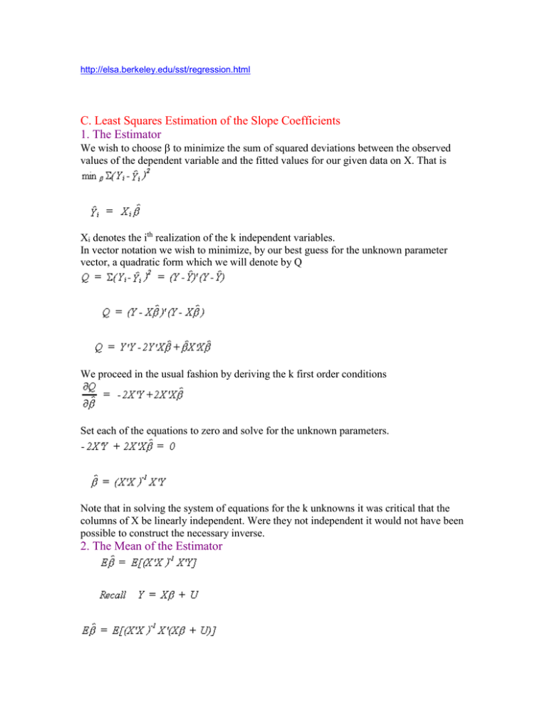
http://elsa.berkeley.edu/sst/regression.html
C. Least Squares Estimation of the Slope Coefficients
1. The Estimator
We wish to choose  to minimize the sum of squared deviations between the observed
values of the dependent variable and the fitted values for our given data on X. That is
Xi denotes the ith realization of the k independent variables.
In vector notation we wish to minimize, by our best guess for the unknown parameter
vector, a quadratic form which we will denote by Q
We proceed in the usual fashion by deriving the k first order conditions
Set each of the equations to zero and solve for the unknown parameters.
Note that in solving the system of equations for the k unknowns it was critical that the
columns of X be linearly independent. Were they not independent it would not have been
possible to construct the necessary inverse.
2. The Mean of the Estimator
We should note several things: Expectation is a linear operator. The error term is
assumed to have a mean of zero. X'X cancels with its inverse. Initially we assumed that X
is non-stochastic. So
The least squares estimator is linear in Y, and by substitution it is linear in the error
term. It is also unbiased.
3. The Variance of the Estimator
Our starting point is the definition of the variance of any random variable.
Substituting in from the expression for the mean of the parameter vector
Again, since the X are non-stochastic and expectation is a linear operator we can cut
right to the heart
4. The Gauss Markov Theorem
We now come to one of the simpler and more important theorems in econometrics. The
Gauss-Markov Theorem states that in the class of linear unbiased estimators the OLS
estimator is efficient. By efficient we mean that estimator with the smallest variance in its
class.
Theorem
If (X) = k where X: nxk,
E(U) = 0 and E(UU')=2I
then
is BLUE.
Proof:
We seek an estimator * that is a linear unbiased estimator with a smaller variance than
the OLS estimator.
Let * = C*Y be an arbitrary linear estimator. Since this is a linear estimator and OLS is
a linear estimator we can choose C* to be a combination of the design matrix. Namely,
C* = C + (X'X)-1X'.
As before Y = X + U.
For * to be unbiased we must impose the restriction that CX = 0. Now from the
definition of variance and using the fact that our new estimator is unbiased we have
Var(*) = E(* - )(* - )'. Or, substituting in for *
But we already know CX = X'C' = 0 so


*)  Var()