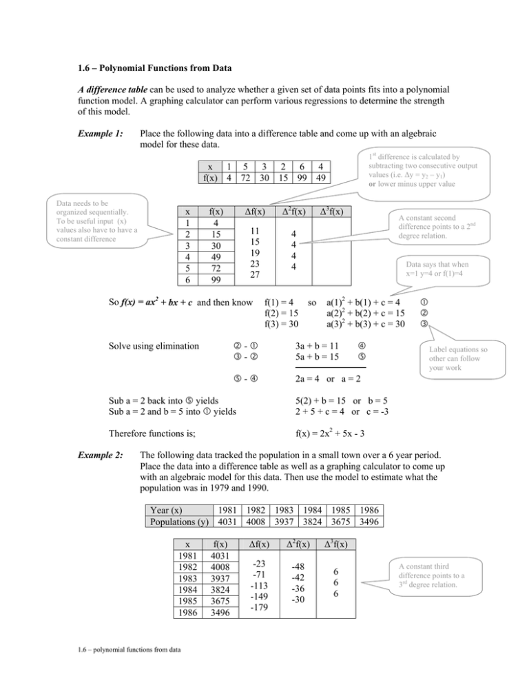
1.6 – Polynomial Functions from Data
A difference table can be used to analyze whether a given set of data points fits into a polynomial
function model. A graphing calculator can perform various regressions to determine the strength
of this model.
Example 1:
Place the following data into a difference table and come up with an algebraic
model for these data.
1st difference is calculated by
subtracting two consecutive output
values (i.e. Δy = y2 – y1)
or lower minus upper value
x 1 5 3 2 6 4
f(x) 4 72 30 15 99 49
Data needs to be
organized sequentially.
To be useful input (x)
values also have to have a
constant difference
x
1
2
3
4
5
6
f(x)
4
15
30
49
72
99
Δf(x)
Δ2f(x)
11
15
19
23
27
4
4
4
4
So f(x) = ax2 + bx + c and then know
Solve using elimination
f(1) = 4
f(2) = 15
f(3) = 30
Δ3f(x)
A constant second
difference points to a 2nd
degree relation.
Data says that when
x=1 y=4 or f(1)=4
so
a(1)2 + b(1) + c = 4
a(2)2 + b(2) + c = 15
a(3)2 + b(3) + c = 30
d-c
e-d
3a + b = 11
5a + b = 15
f
g
g-f
2a = 4 or a = 2
Sub a = 2 back into g yields
Sub a = 2 and b = 5 into c yields
5(2) + b = 15 or b = 5
2 + 5 + c = 4 or c = -3
Therefore functions is;
f(x) = 2x2 + 5x - 3
Example 2:
c
d
e
Label equations so
other can follow
your work
The following data tracked the population in a small town over a 6 year period.
Place the data into a difference table as well as a graphing calculator to come up
with an algebraic model for this data. Then use the model to estimate what the
population was in 1979 and 1990.
Year (x)
1981 1982 1983 1984 1985 1986
Populations (y) 4031 4008 3937 3824 3675 3496
x
1981
1982
1983
1984
1985
1986
1.6 – polynomial functions from data
f(x)
4031
4008
3937
3824
3675
3496
Δf(x)
Δ2f(x)
Δ3f(x)
-23
-71
-113
-149
-179
-48
-42
-36
-30
6
6
6
A constant third
difference points to a
3rd degree relation.
Difference table show a 3rd degree relation which is confirmed by a regression value of 1
on the graphing calculator
So we know it will have the general form:
p(y) = ay3 + by2 + cy + d
The graphing calculator gives the following:
a=1
b = -5970
c = 11880060
d = -7880118800
R value indicates a
strong postive
correlation
So our equation is:
And so 1979
R2 = 1
Large values would
make algebraic
calculation more
difficult. One could
adjust years to zero
(i.e. 1981Æ0 and
1982Æ 1, etc)
p(y) = y3 – 5970y2 + 11880060y - 7880118800
p(1979) = (1979)3 – 5970(1979)2 + 11880060(1979) - 7880118800
= 3909
p(1990) = 2600
Population as a
function of year
1.6 – Polynomial Functions from Data Practice Questions
1. Determine, by algebraic methods, a polynomial function that models the data below;
a)
b)
c)
d)
(1,0), (2,-2), (3,-2), (4,0), (5,4), (6,10)
(1,-1), (2,2), (3,5), (4,8), (5,11), (6,14)
(1,-4), (2,0), (3,30), (4,98), (5,216), (6,396)
(1,-9), (2,-10), (3,-7), (4,0), (5,11), (6,26)
2. Use a graphing calculator to determine the best polynomial function that models the data.
Note that the data does not necessarily have a perfect (regression value of 1) fit to one
polynomial model
a) (1,1), (2,-3), (3, 5), (4,37), (5,105), (6,221)
b) (0,4), (1,16), (2,30), (3,60), (4,120), (5,250)
c) (1,-9), (2,-31), (3,-31), (4,51), (5,299), (6,821)
Answers 1. a) f(x)= x2 - 5x + 4 b) g(x) = 3x - 4 c) h(x) = 2x3 + x2 – 13x + 6 d) m(x) = 2x2 – 7x – 4
2. a) y=2x3-6x2+5 R=1 b) y=3.5x3-12.7x2+24.3x+3.2 R=0.99 c) y=x4-14x2+5x-1 R=1
1.6 – polynomial functions from data