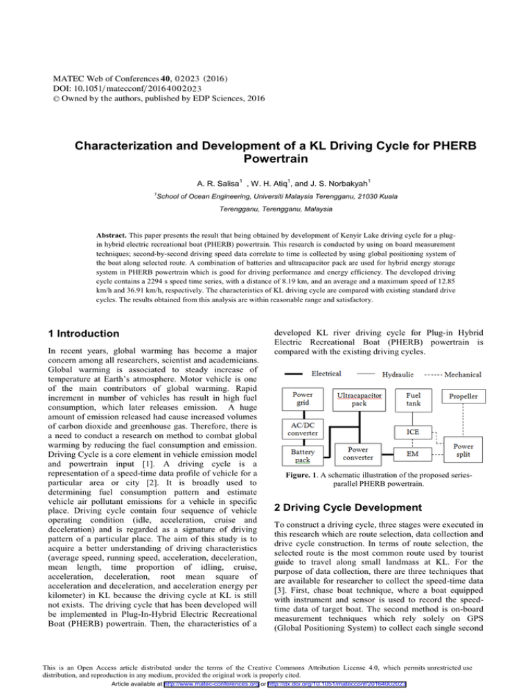
MATEC Web of Conferences 4 0, 0 2 0 23 (2016 )
DOI: 10.1051/ m atecconf/ 2016 4 0 0 2 0 2 3
C Owned by the authors, published by EDP Sciences, 2016
Characterization and Development of a KL Driving Cycle for PHERB
Powertrain
1
1
A. R. Salisa , W. H. Atiq , and J. S. Norbakyah
1
1
School of Ocean Engineering, Universiti Malaysia Terengganu, 21030 Kuala
Terengganu, Terengganu, Malaysia
Abstract. This paper presents the result that being obtained by development of Kenyir Lake driving cycle for a plugin hybrid electric recreational boat (PHERB) powertrain. This research is conducted by using on board measurement
techniques; second-by-second driving speed data correlate to time is collected by using global positioning system of
the boat along selected route. A combination of batteries and ultracapacitor pack are used for hybrid energy storage
system in PHERB powertrain which is good for driving performance and energy efficiency. The developed driving
cycle contains a 2294 s speed time series, with a distance of 8.19 km, and an average and a maximum speed of 12.85
km/h and 36.91 km/h, respectively. The characteristics of KL driving cycle are compared with existing standard drive
cycles. The results obtained from this analysis are within reasonable range and satisfactory.
1 Introduction
In recent years, global warming has become a major
concern among all researchers, scientist and academicians.
Global warming is associated to steady increase of
temperature at Earth’s atmosphere. Motor vehicle is one
of the main contributors of global warming. Rapid
increment in number of vehicles has result in high fuel
consumption, which later releases emission. A huge
amount of emission released had cause increased volumes
of carbon dioxide and greenhouse gas. Therefore, there is
a need to conduct a research on method to combat global
warming by reducing the fuel consumption and emission.
Driving Cycle is a core element in vehicle emission model
and powertrain input [1]. A driving cycle is a
representation of a speed-time data profile of vehicle for a
particular area or city [2]. It is broadly used to
determining fuel consumption pattern and estimate
vehicle air pollutant emissions for a vehicle in specific
place. Driving cycle contain four sequence of vehicle
operating condition (idle, acceleration, cruise and
deceleration) and is regarded as a signature of driving
pattern of a particular place. The aim of this study is to
acquire a better understanding of driving characteristics
(average speed, running speed, acceleration, deceleration,
mean length, time proportion of idling, cruise,
acceleration, deceleration, root mean square of
acceleration and deceleration, and acceleration energy per
kilometer) in KL because the driving cycle at KL is still
not exists. The driving cycle that has been developed will
be implemented in Plug-In-Hybrid Electric Recreational
Boat (PHERB) powertrain. Then, the characteristics of a
developed KL river driving cycle for Plug-in Hybrid
Electric Recreational Boat (PHERB) powertrain is
compared with the existing driving cycles.
Figure. 1. A schematic illustration of the proposed seriesparallel PHERB powertrain.
2 Driving Cycle Development
To construct a driving cycle, three stages were executed in
this research which are route selection, data collection and
drive cycle construction. In terms of route selection, the
selected route is the most common route used by tourist
guide to travel along small landmass at KL. For the
purpose of data collection, there are three techniques that
are available for researcher to collect the speed-time data
[3]. First, chase boat technique, where a boat equipped
with instrument and sensor is used to record the speedtime data of target boat. The second method is on-board
measurement techniques which rely solely on GPS
(Global Positioning System) to collect each single second
This is an Open Access article distributed under the terms of the Creative Commons Attribution License 4.0, which permits XQUHVWULFWHGXVH
distribution, and reproduction in any medium, provided the original work is properly cited.
Article available at http://www.matec-conferences.org or http://dx.doi.org/10.1051/matecconf/20164002023
MATEC Web of Conferences
are used to analyse and characterize KL driving cycle
speed-time data as listed in Table I. Fig. 2 present the
flowchart regarding the stages of data analysis and
development of driving cycle. The selected route for KL
driving cycle development is illustrated in Fig. 3.
of speed-time data. The third method is combination of
both techniques. However, this study only adopts the
second method since there are insufficient expert boat
driver to undertake the chase boat method. Besides, the
second method can minimize the possibility of boat
accident. According to the past study [4 – 5], 12 variables
Table 1. Variables Used in KL Driving Cycle Analysis
No
Variable
Unit
v1
1
Average Speed ,
2
Average Running Speed,
3
4
Average Acceleration,
Average Deceleration,
Formula
dist
T total
dist
v _ run 3.6
T drive
v _ avg 3.6
km/h
v2
km/h
a
2
m/s
d
2
m/s
n 1 (a 0) a _ avg i
i 1 0 (else) 1
n 1 (a 0) d _ avg i
0
(else)
i
1
1
1 (a i 0)
n
0
i 1
(else)
1 (a i 0)
n
0
i 1
(else)
n
5
c
Mean Length of a driving period,
s
6
Time Proportion of Idling,
Pi
%
7
Time Proportion of Cruise,
Pc
%
8
Time Proportion of Acceleration,
pa
%
9
Time Proportion of Deceleration,
Pd
%
10
11
T totalt 2 t 1 (t i t i 1)
i 2
T drive
T total
T
%cruise cruise
T total
T
%acc acc
T total
T
%dec dec
T total
%drive Average number of acceleration-deceleration
changes within one driving period,
M
Root Mean Square of Acceleration, RMS
-
m/s2
RMS 1
T total
Acceleration Energy per Kilometer,
KPE
m/s2
02023-p.2
PKE a
2
i
i 1
1 n v i vi21 (v i v i 1)
dist i 2 (else)
2
12
n
ICMES 2015
Figure. 2. Flow chart of Kenyir Lake Driving Cycle Development
Figure. 3. The selected route of Kenyir Lake
02023-p.3
MATEC Web of Conferences
3 Data Analysis
The data is collected during the period of 10:00-12:00p.m
for 20 days on April 2015. One run is handled to record
one data per day. In the end 20 run was collected. SpeedTime data is collected by using Global Positioning
System along the selected route around KL. The value of
12 data variables which has been used in conducting the
speed-time data analysis is shown in Table 2. The mean
values in Table 3 are obtained from Table 2. The mean
value from table 3 has been calculated by summation of
data in table 2 which was divided by 20 runs. After the
mean value is gained, the percentage error for all run is
calculated in Table 4. In the Table 5 it shown the most
minimum percentage error is from Run 9 that has been
calculated in the Table 4. Run 9 is the one with the
smallest percentage error is considered as the best KL
drive cycle. The average speed for KL is 12.85 km/h and
the average running speed is 12.91 km/h. The results
indicated that the speed is very slow. For complete
circulation at KL, the rate for acceleration and
deceleration is equal which is 0.35.The four vehicle
operating modes is calculated. The time proportion of
idling, time proportion of cruising, time proportion of
acceleration and time proportion of deceleration are
0.44 %, 0.70 %, 49.54 % and 49.37 % respectively. The
value of total time and mean length of driving period is
equal, that is 2294s. When the driving period is close or
equal to total time, it showed that the driving period is
high, and it indicates that the route is clear and there is no
obstacle along the path. The Root Mean Square for this
run is 0.43 and the Acceleration Energy per Kilometer is
0.35. The best KL driving cycle is constructed as
presented in Fig. 4.
Table 2. KL driving cycle data analysis
Pi
Pc
pa
Pd
(%)
(%)
(%)
(%)
5
6
7
8
0.27
2275
0.53
0.04
0.28
0.29
2307
0.61
12.90
0.27
0.27
2295
12.89
12.98
0.26
0.26
…..
…..
…..
12.85
12.91
Run …..
…..
Run 17
d
M
RMS
KPE
9
10
11
12
50.22
49.34
1.00
0.34
0.28
0.04
50.61
48.87
0.99
0.36
0.28
0.39
0.04
49.74
49.96
1.00
0.35
0.28
2252
0.67
0.44
49.67
49.27
0.99
0.34
0.27
…..
…..
…..
…..
…..
…..
…..
…..
…..
0.35
0.35
2294
0.44
0.70
49.54
49.37
0.99
0.43
0.35
…..
…..
…..
…..
…..
…..
…..
…..
…..
…..
…..
12.93
12.98
0.36
0.35
2274
0.44
0.22
49.10
50.29
0.99
0.46
0.37
Run 18
13.02
13.08
0.36
0.37
2299
0.48
0.74
50.39
48.43
0.99
0.45
0.37
Run 19
12.85
12.92
0.35
0.34
2264
0.57
1.72
48.17
49.58
0.98
0.44
0.34
Run 20
12.89
12.95
0.36
0.36
2280
0.48
0.31
50.24
49.01
0.99
0.45
0.37
M
RMS
KPE
v1
v2
(km/h)
(km/h)
(m/s2 )
(m/s2 )
(s)
j
1
2
3
4
Run 1
12.93
13.00
0.26
Run 2
12.99
13.07
Run 3
12.85
Run 4
Run …..
Criterion
Run 9
a
c
(m/s2 )
(m/s2 )
Table 3. Mean values of the assessment parameters of grouped runs
Criterion
j
Mean
Value
Route 1
(run 1 –
run 20)
a
Pi
Pc
pa
Pd
(%)
(%)
(%)
(%)
5
6
7
8
9
10
11
12
2280.45
0.50
0.56
47.25
49.33
0.99
0.42
0.34
c
v1
v2
(km/h)
(km/h)
(m/s2 )
(m/s2 )
(s)
1
2
3
4
12.92
12.99
0.33
0.33
d
02023-p.4
(m/s2 )
(m/s2 )
ICMES 2015
Table 4. Percentage difference relative to target summary statistics
a
v1
v2
(km/h
)
(km/h
)
(m/s2
)
(m/s2
)
J
1
2
3
Mean
Value
12.92
12.99
Run 1
0.08
Run 2
d
KPE
(m/s2 )
(m/s2 )
10
11
12
49.3
3
0.9
9
0.42
0.34
6.29
0.02
1.0
1
19.05
17.65
182.6
7
92.86
7.11
0.93
0
14.29
17.65
184.4
3
22.0
0
92.86
5.27
1.28
1.0
1
16.67
17.65
194.9
7
1.25
34.0
0
21.43
5.12
0.12
0
19.05
20.59
144.2
9
…..
…..
…..
…..
…..
…..
…..
…..
…..
…..
6.06
6.06
0.59
12.0
0
25.00
4.85
0.08
0
2.38
2.94
61.12
…..
…..
…..
…..
…..
…..
…..
…..
…..
…..
…..
…..
0
0.08
9.09
12.12
0.37
12.0
0
55.36
5.08
0.51
0
9.52
5.88
110.0
1
0.08
0.08
9.09
6.06
0.28
12.0
0
60.71
3.92
1.95
0
9.52
8.82
112.5
1
0.77
0.69
9.09
12.12
0.81
4.00
32.14
6.65
1.82
0
7.14
8.82
0.54
0.54
6.06
3.03
0.72
14.0
0
207.1
4
1.95
0.51
1.0
1
4.76
0
0.23
0.31
9.09
9.09
0.02
4.00
44.64
6.33
0.65
0
7.14
8.82
(s)
Pc
pa
Pd
(%)
(%)
(%)
(%)
4
5
6
7
8
9
0.33
0.33
2280.4
5
0.50
0.56
47.2
5
0.08
21.21
18.18
0.24
6.00
92.86
0.54
0.62
15.15
12.12
1.16
22.0
0
Run 3
0.54
0.69
18.18
18.18
0.64
Run 4
0.23
0.08
21.21
21.21
Run …..
…..
…..
…..
Run 9
0.54
0.62
Run …..
…..
Run 16
Run 17
Run 18
Run 19
Run 20
Total
Error
(%)
RMS
Pi
Criterio
n
c
M
84.05
240.2
6
90.32
Table 5. Minimum Percentage Error of the Assessment Parameters of grouped runs
a
Pi
Pc
pa
Pd
(%)
(%)
(%)
(%)
5
6
7
8
0.59
12.00
25.00
4.85
c
v1
v2
(km/h)
(km/h)
(m/s2 )
(m/s2 )
(s)
J
1
2
3
4
Run 9
0.54
0.62
6.06
6.06
Criterion
d
02023-p.5
M
RMS
KPE
9
10
11
12
0.08
0
2.38
2.94
(m/s2 )
(m/s2 )
Total Error
(%)
61.12
MATEC Web of Conferences
Figure. 4. The Kenyir Lake drive cycle
4 Conclusion
Based on the results of this study, it can be concluded that
the proposed method is possible to generate a KL driving
cycle for PHERB powertrain in order to measure fuel
consumption and emissions and it was proved by the
tabulate data above. This paper also proved that from
executed research above that there is potential ability to
use this data on PHERB powertrain.
2.
Acknowledgment
4.
The financial support of this work by the Fundamental
Research Grant Scheme and the Universiti Malaysia
Terengganu, is gratefully acknowledged.
5.
3.
References
1. Kamble, S.H., Mathew, T.V., & Sharma, G. (2009).
02023-p.6
Development of real world driving cycle:
Case study of Pune, India. Transportation Research
Part D, 132-140.
W.T. Hung, H.Y.Tong, C.P. Lee, K.Ha, & L.Y. Pao.
(2007). Development of a
Practical Driving
Cycle Construction Methodology: A Case Study in
Hong Kong. Transportation Research Part D, Vol.
12, pp. 115–128.
Z. Xiao, Z. D. Jia and S. J. Min. (2012) A Synthesis
of Methodologies and Practices for Developing
Driving Cycles. Energy Procedia 16, pp. 1868-1873.
Hung, W.T., Tong, H.Y., Lee, C.P., Ha, K., & Pao,
L.Y. (2007).Development of a practical driving cycle
construction methodology: A case study in Hong
Kong. Transportation Research Part D, 132-140.
T. J. Barlow, S. Latham, I. S. McCrae and P. G.
Boulter, “A Reference Book of Driving Cycles for
Use in the Measurement of Road Vehicle Emissions”,
published project report PPR354 for the Department
for Transport, version 3, June 2009.