The Workshops of the Thirtieth AAAI Conference on Artificial Intelligence
Expanding the Boundaries of Health Informatics Using AI:
Technical Report WS-16-08
Combining Multiple Concurrent Physiological Streams
to Assessing Patients Condition
Shenda Hong, Zhen Qiu, Jinbo Zhang and Hongyan Li ∗
Key Laboratory of Machine Perception, Ministry of Education
School of EECS, Peking University, Beijing, 100871, China
{hongshenda, qiuzhen, zhangjinbo, lihy}@cis.pku.edu.cn
Abstract
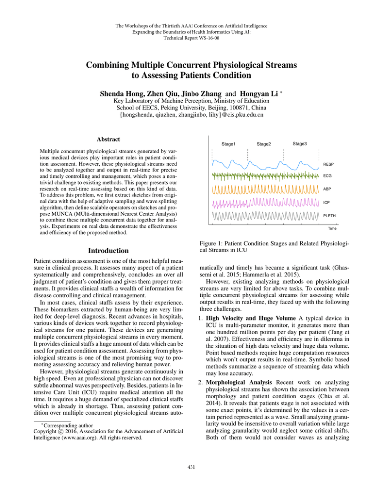
Stage1
Multiple concurrent physiological streams generated by various medical devices play important roles in patient condition assessment. However, these physiological streams need
to be analyzed together and output in real-time for precise
and timely controlling and management, which poses a nontrivial challenge to existing methods. This paper presents our
research on real-time assessing based on this kind of data.
To address this problem, we first extract sketches from original data with the help of adaptive sampling and wave splitting
algorithm, then define scalable operators on sketches and propose MUNCA (MUlti-dimensional Nearest Center Analysis)
to combine these multiple concurrent data together for analysis. Experiments on real data demonstrate the effectiveness
and efficiency of the proposed method.
Stage2
Stage3
RESP
ECG
ABP
ICP
PLETH
Time
Figure 1: Patient Condition Stages and Related Physiological Streams in ICU
Introduction
Patient condition assessment is one of the most helpful measure in clinical process. It assesses many aspect of a patient
systematically and comprehensively, concludes an over all
judgment of patient’s condition and gives them proper treatments. It provides clinical staffs a wealth of information for
disease controlling and clinical management.
In most cases, clinical staffs assess by their experience.
These biomarkers extracted by human-being are very limited for deep-level diagnosis. Recent advances in hospitals,
various kinds of devices work together to record physiological streams for one patient. These devices are generating
multiple concurrent physiological streams in every moment.
It provides clinical staffs a huge amount of data which can be
used for patient condition assessment. Assessing from physiological streams is one of the most promising way to promoting assessing accuracy and relieving human power.
However, physiological streams generate continuously in
high speed. Even an professional physician can not discover
subtle abnormal waves perspectively. Besides, patients in Intensive Care Unit (ICU) require medical attention all the
time. It requires a huge demand of specialized clinical staffs
which is already in shortage. Thus, assessing patient condition over multiple concurrent physiological streams auto-
matically and timely has became a significant task (Ghassemi et al. 2015; Hammerla et al. 2015).
However, existing analyzing methods on physiological
streams are very limited for above tasks. To combine multiple concurrent physiological streams for assessing while
output results in real-time, they faced up with the following
three challenges.
1. High Velocity and Huge Volume A typical device in
ICU is multi-parameter monitor, it generates more than
one hundred million points per day per patient (Tang et
al. 2007). Effectiveness and efficiency are in dilemma in
the situation of high data velocity and huge data volume.
Point based methods require huge computation resources
which won’t output results in real-time. Symbolic based
methods summarize a sequence of streaming data which
may lose accuracy.
2. Morphological Analysis Recent work on analyzing
physiological streams has shown the association between
morphology and patient condition stages (Chia et al.
2014). It reveals that patients stage is not associated with
some exact points, it’s determined by the values in a certain period represented as a wave. Small analyzing granularity would be insensitive to overall variation while large
analyzing granularity would neglect some critical shifts.
Both of them would not consider waves as analyzing
∗
Corresponding author
c 2016, Association for the Advancement of Artificial
Copyright Intelligence (www.aaai.org). All rights reserved.
431
units.
3. Concurrency and Correlation The human body is a
complex integration of physiological and pathological
processes. Most biological processes are mutually correlated and bound together by physical or physiological control and communication phenomena. Analyzing
any single process may only provide partial information
and pose difficulties in the comprehension of the process. Physiological streams from various sources including hearts, brains and endocrine require researchers consider every physiological stream concurrently to obtain
the complete information. Thus, simply implement methods of single stream in the multiple streams condition repeatedly would get bias results or even contradictory results.
To address these challenges, this paper propose a novel assessing approach for multiple physiological streams. We first
introduce an adaptive sampling algorithm to keep a balance
between efficiency and effectiveness. Then choose waves
as our concerned granularity and use sketches to represent
the outline of original data. Finally, we develop MUNCA
(MUlti-dimensional Nearest Center Analysis) to combine
sketches of various streams together for analysis. Experiments on real data demonstrate the effectiveness and efficiency of the proposed method.
The rest of the paper is organized as follows. First, we
describe preliminaries and give an overview of our work.
Physiological sketches extraction is introduced afterwards.
After we present assessing method based on sketches, we
show experiments on our approach. And then we introduce
the related work. Lastly, we conclude the research and gives
directions for future studies.
Figure 2: Framework
3. Critical shifts appear from one wave to another are considered significant.
Based on that, we propose our approach illustrated in
Fig.2. Our goal is to give current stage Y (t) based on multiple medical streams. We first extract sketches using adaptive sampling and wave splitting algorithm; Then we split
each data streams into meaningful waves; Next, we build our
assessing method MUNCA and implement online learning.
Finally, we can assess current stage over medical streams in
real-time.
Physiological Sketches Extraction
It’s critical to extract useful information from such a huge
amount of high speed data streams. In this section, we propose a suite of approaches to effectively compress the data
while keep the outline of the original data, and split sampled
data to get sketches (can be regard as features) for further
analysis.
Preliminaries
In this section, we formally define the problem of assessing
over multiple physiological streams, and describe the framework of our method.
Adaptive Sampling
Definition 1. (Multiple Concurrent Physiological Streams):
Let {S (1) (t), S (2) (t), ..., S (N ) (t)} denote N source multiple physiological streams that are all associated with one
patient.
To achieve real-time assessing, it’s indispensable to extract
a fraction of points from original data while keeping the outline. A widely used way is sampling in fixed interval from
original data. It’s simple and convenient but would lead to
concept drifting due to the pseudo periodicity of physiology
streams. Advanced methods like PLR (Tang et al. 2007) and
SAX (Lin et al. 2003) have the computational complexity of
O(n2 ), which are not satisfied with real-time assessing. Others like PIP (Fu et al. 2008) only capture the local extreme
points which is insensitive to overall variation.
An adaptive way is to associate sampling interval with
variation magnitude represented by derivative. However, we
can’t calculate derivative from streaming data directly since
thses discrete points can’t deduce derivative function. A feasible solution is to use absolute numerical central differentiation to approximate actual derivative as Eq.1 shows. The
accuracy can reach to O(∆t)4 .
we use ∆t represent sample time interval. Then we can
get that S (d) (t0 + ∆t) is the next point of S (d) (t0 ) in dth
stream. For simplicity, we use S(ti ) or S(t) to represent one
of the physiological streams in this section, other streams are
handled similarly.
Definition 2. (Stage): Let Y (t) denote the stage function,
Y (t) ∈ {Y1 , Y2 , ...YL }, the codomain is a finite set of nominal value, which indicate various conditions of a patient.
Some key properties in multiple concurrent physiological
streams include (Tang et al. 2007):
1. The morphology of waves are similar in a certain stage of
all people;
2. The morphology of waves are dissimilar in different
stages of all people;
D(t) =
432
−S(t + 2∆t) + 8S(t + ∆t) − 8S(t − ∆t) + S(t − 2∆t)
12∆t
(1)
Original Data
Original data
Processed Data
Edge Point
PAA
Adaptive
Figure 3: Adaptive Sampling
Figure 4: Wave Splitting
Intuitively, we want to increase sampling density as D(t)
increasing, and decrease sampling density as D(t) decreasing. We choose sampling timestamp ti using formula:
4) Divide by edge points. We detect elbow points in processed streams as split position in original streams.
The computational complexity of splitting is O(M n).
ti = ti−1 + b
β
c∆t
|D(t)|
Aligning Sketches
(2)
After splitting, we get series of subsequences represents
each stream of all multiple concurrent streams. These subsequences are defined as sketches.
s(i) = S(ti )
Where β is a parameter controlling sampling density, s(i)
is sampled data and S(ti ) is original data. The computational
complexity of sampling is O(n).
Definition 3. (Sketch): Some key points sequence that keep
the outline of the original waves. The ith sketch in jth de(i)
vices denote as skj .
Wave Splitting
Besides, aligning sketches in each stream to conduct a
batch of input shouldn’t be ignored. We choose the first
stream as standard timestamp, and align sketches’ timestamp in other streams.
To get waves for analyzing, we should split each long
term stream of multiple concurrent streams into consecutive waves. However, simply dividing data streams in fixed
length will accumulate error leading to concept drifting due
to the inequality of consecutive waves. Besides, dividing
streams into waves at the key points directly will also divide the critical shift into separated parts. To weakening the
disturbance of noise and long-term trend while maintaining
integrity of waves and critical shifts, while finding split position correctly. It can be achieved by following steps:
1) Differentiation. To obtain information on critical shifts
and overcome the concept drift problem.
Multi-dimensional Nearest Center Analysis
In this section, we will introduce MUNCA and implement it
on these aligned batches of sketches to get assessed stages.
Scalable Operators on Sketch
After preprocessing, the length of sketches are not the same
in most cases. Normal operations can not be applied in Euclid space on different length vectors. A common solution is
to truncate the longer sketch to the shorter one, or padding
the shorter sketch to the longer one. It may lose importance
feature on sketches, or adding nonsense sequence. Another
solution is to embed sketches into a lower dimensional space
using Multidimensional Scaling (MDS) (Young 2013), but it
requires heavy computation.
Thus, computation on sketches require special operators
that can handle with scalable situation. Inspired by warping path in Dynamic Time Warping (Rakthanmanon et al.
2012), we denote an elastic projection from one sketch to
another. For formal definition, a m length sketch si =
(x1 , x2 , ..., xm ) and a n length sketch sj = (y1 , y2 , ..., yn ).
then we can get a projection from each point from si to sj ,
vise versa.
S(t + ∆t) − S(t − ∆t)
(3)
2∆t
2) Squaring operation. To amplify the magnitude of critical shifts while makes all data points positive.
S(t) =
S(t) = S(t)2
(4)
3) Moving average filter. To reduce noise and smooth fluctuation.
S(t) + S(t − ∆t) + ... + S(t − (M − 1)∆t)
M ∆t
(5)
Where M ∆ t is the length of moving average.
S(t) =
433
can deduce the following equation:
G(S) = argmaxP (Y | S)
Y
= argmaxP (S | Y )P (Y )
Y
(14)
= argmax
Y
(6)
Psj (si ) = (x01 , x02 , ..., x0n )
(7)
G(S) = argmax
Y
(11)
0 )2
(x1 − y10 )2 + (x2 − y20 )2 + ... + (xm − ym
(12)
Where c is a real number, × is normal times operator.
Implementing Online MUNCA
We regard stage function Y (t) as a random variable. Since
stage Y is a finite nominal value, it’s natural that we assume
stage Y is obeying multinomial distribution. Besides, the
distribution of sketches should be around a ”center” sketch
in a particular stage. So we also assume each sketch S (d) in
stream S (d) (t) obeying gaussian distribution given stage Y ,
while these distributions are independent and their covariance matrix are all the same.
Y ∼ M ultiN ominal(p1 , p2 , ..., pL )
S
(d)
| Y = l ∼ N (µl , Σ)
e−||S
(d)
2
µY ||2
P (Y )
(16)
d=1
Algorithm 1 Updating Center and Probability of Y
1: Input: S, center, step, P (Y ), Ytrue
2: Output: center, step, P (Y )
3: for d = 1 to N do
4:
candi1=(S (d) ⊕ (step − 1)center(d) )/step
5:
candi2=((step − 1)center(d) ⊕ S (d) )/step
2
2
6:
dist1 = ||cand1 S (d) ||2 + ||cand1 center(d) ||2
2
2
7:
dist2 = ||cand2 S (d) ||2 + ||cand2 center(d) ||2
8:
if dist1 ≤ dist2 then
9:
center(d) = dist1
10:
else
11:
center(d) = dist2
12:
end if
13: end for
14: P (Ytrue ) = P (Ytrue ) + 1/step
15: step = step + 1
16: return center, step, P (Y )
Note that Commutative Laws is false here because we get
different length result if the sketches order are shifted.
The following equations can be easily proofed:
p
N
Y
Note that each sketch S (d) obeying gaussian distribution
given stage Y with the same covariance matrix Σ. So we
can assign S to stage Y which has the most probability as
Eq.16 shows. Intuitively, we actually assign each S (d) to the
nearest center.
Then we will implement our method as online learning in
Algorithm 1.
0
si ⊕ (sj ) = si + Psi (sj ) = (x1 + y10 , x2 + y20 , ..., xm + ym
)
(8)
0
si (sj ) = si − Psi (sj ) = (x1 − y10 , x2 − y20 , ..., xm − ym
)
(9)
0
si ⊗ (sj ) = si × Psi (sj ) = (x1 × y10 , x2 × y20 , ..., xm × ym
)
(10)
||si sj ||2 =
d=1
Then we can simply deduce Eq.16 based on our assumption.
Note that we project n length sketch sj to m length in
Eq.6.
Then we define plus operation ⊕, minus operation and
times operation ⊗ on sketch:
c × si = (cx1 , cx2 , ..., cxm )
P (S (d) | Y )P (Y )
According to Eq.13, P (S (d) | Y ) obeys the normal distribution:
(d)
T −1
(d)
1
e−(S µY ) Σ (S µY )
P (S (d) | Y ) = √ n/2
1/2
2π |Σ|
(15)
Figure 5: Projection based on DTW
0
Psi (sj ) = (y10 , y20 , ..., ym
)
N
Y
Accoding to Eq.16, the assessing result is only determined
by the center (Expectation) µY and probability of stage Y.
So we only have to store µY and P (Y ) for assessing, and
update them every time when a new batch of sketches is
coming. Finally, we can apply Eq.16 using updated µY and
P (Y ) for assessing.
Note that MUNCA is working on the sketches instead
of original data. The computational complexity is O(L2 m),
where L is the codomain size of Y (t), m is the average
length of sketch. So the computational complexity of the
whole procedure is still O(n).
(13)
Our goal is to assess stage Y based on a batch of sketches
S. We use P (S|Y ) denote the probability of S in stage Y ,
and use G(S) denote the assessing result given S. And we
434
Experiments
Accuracy (%)
100
In this section, we conduct a thorough experiments on our
method. First we evaluate some issues that affect the performance of proposed method, then we compare it with some
existing methods.
80
60
Less than 0.1% points of the entire dataset
40
Experimental Settings
20
We use real datasets instead of synthetic datasets. Two kinds
of multiple streams are used in the experiments:
0
0
5
10
15
20
25
Points
(unit:104)
Figure 6: Learning Velocity
1. MIT-BIH Arrhythmia Database Directory (MITDB)
(Goldberger et al. 2000): Two-channel ambulatory ECG
recordings contains over 4000 long-term Holter recordings which obtained from inpatients who have premature
beats. The stage include Premature ventricular contraction
(represent as V) and Normal beat (represent as N)
To further see how the size of sketches affect the assessing
accuracy, we also carried out experiments on our adaptive
sampling algorithm. As shown in Fig.7, with sketches size
increasing, the similarity of sketches and original waves is
also increasing, leading to the promotion of assessing accuracy. When the size of sketches is about 10% of the original waves in average, the assessing accuracy is steady which
means that sketches are very close to original waves. The elbow point is 7.9% of the original waves in average, which
is the best sketch size choice for achieving good efficiency
while keep rational accuracy. And the parameter β is set to
29.05, So we choose it for all of our experiments in ICU
dataset.
2. ICU Dataset (ICU) (Tang et al. 2007): Five real physiological streams from multi-parameter monitor including
RESP, ECG, ABP, ICP, PLETH are recorded during a six
hour period simultaneously from a pediatric patient with
traumatic brain injury. The stage include mild (M), severe
(S) and emergency (E). The sample rates of the signals are
from 125 Hz to 500 Hz, and the whole dataset includes
over 25,000,000 data points;
Accuracy (%)
100
The experiments were conducted on the hardware configuration with 4-core 2.90GHz Intel CPU and 8GB memory
running MATLAB R2014a in Windows 7 Professional.
80
Method Performance
Elbow Point
60
The first experiment carried out on the ICU Dataset is to test
the effectiveness of online learning. As introduced before,
we implement MUNCA as online learning style. So it’s important to see how fast online learning style achieve a comparable accuracy with training-testing style. Fig.6 shows the
learning velocity of MUNCA. We chose sampling density
parameter β as 29.05 which will explained later. The straight
horizontal line is the accuracy of training testing style (20%
training). We can see that online MUNCA achieves rapid
accuracy gain from zero to 80% within processing about
10, 000 points, which is less than 0.1% of the entire dataset.
As more data processed, online learning style is even better
than training testing style. The reason is that online learning
style can adjust model timely when new data coming. Besides, the big accuracy promotion is because MUNCA only
update sketches instead of the original data, which reduce
the computational complexity remarkably.
40
20
0
5
10
15
20
25
Percent of the original data (%)
Figure 7: Sketch Size vs Assessing Accuracy
Comparison with Other Methods
As we illustrated in Related Work, these assessing method
can be loosely divided into three categories. To get a comprehensive result, we compared our method with three most
relevant methods from three categories: Regression(Chen et
al. 2002) (point based), FastShapelet(Keogh and Rakthan-
435
Accuracy (%)
Point Processed per Second
100
80
MITDB
60
Regression
SAX
FastShapelet
MUNCA
40
Regression
SAX
FastShapelet
MUNCA
20
ICU
0
MITDB
0
5000
10000
15000
20000
ICU
25000
Figure 9: Assessing Accuracy
Figure 8: Processing Efficiency
Related Work
Most of the existing assessing methods are based on single
physiological stream. Some can handle with multiple physiological streams. These techniques can be loosely divided
into three categories:
A number of assessing method are point based analysis.
In (Chen et al. 2002), they investigated regression method
to analyze streaming data. (Huang et al. 2014) used critical
points to assess from multiple medical sensor data streams.
(Torres and Aguilar-Ruiz 2014) and (Chen, Zou, and Tu
2012) built similarity-based approaches to estimate the distance for assessing. (Rutkowski et al. 2014) applied decision
trees for assessing the class of data streams. These methods
assess stage over exact value of points directly, so they are
slow on large volume data streams, and they don’t take the
morphology of waves into consideration.
Another category of work is wave based analysis, they
split to get the waves and assess stage based on the morphology of waves. (Ye and Keogh 2011) used prototypical
snippets called Shapelet to classify unlabeled streams within
some previously learned distance threshold. It achieves superior accuracy on many datasets but its computational complexity is cubic and intractable on large datasets. So in
(Keogh and Rakthanmanon 2013), they sped up Shapelet
to quadratic running time while keeping accuracy. But both
of them still focus on single stream, they can’t handle with
multiple data streams concurrently. (McGovern et al. 2011)
introduced motif to multiple data streams. But concurrent
motifs are very rare in multiple data streams so it can’t give
results in most cases.
Besides, some methods use symbol to represent a sequence of points, then assess stage based on symbols’ semantics. (Yeh, Dai, and Chen 2007) and (Tang et al. 2007)
used piecewise linear regression to fit a sequence of points
and get the symbol. SAX (Lin et al. 2003) is a widely used
representation method, and has implemented in financial
markets (Canelas, Neves, and Horta 2013), computer vision
(Junejo and Aghbari 2012), etc. These symbolic methods
would neglect some critical shifts and they still not consider
manon 2013) (wave based) and SAX(Lin et al. 2003) (symbolic based).
The first experiment is about processing efficiency. We
implemented these four methods both on MITDB dataset
and ICU dataset. The average numbers of data points processed per second are illustrated in Fig.8. The result shows
that the Regression has the slowest procession speed because it takes every point as concerned granularity. SAX and
FastShapelet perform better than Regression, because they
take waves (FastShapelet) or a sequence of points (SAX) as
concerned granularity. Similarly, MUNCA takes waves into
analysis but it still performs much better than FastShapelet.
The main reason is that MUNCA also use sketches to represent waves, which remarkably reduce computational complexity for the assessing procedure.
At last, we compared assessing accuracy between these
four methods. We compared the assessing result with the
true stage Y(t) to evaluate the accuracy. As SAX and
FastShapelet can’t handle with assessing on multiple data
streams concurrently. We implemented them on each stream
of these multiple streams, and chose the best accuracy as
the result. The assessing accuracy is shown in Fig.9. The result indicates that the Regression performs worse than three
other methods. The reason is that it takes every point into
analysis while the value of stage is actually related to the
morphology of a wave, not the exact value of the points.
SAX is better than regression but still much worse than FastShapelet and MUNCA. The accuracy of MUNCA is better
than FastShapelet in MITDB dataset while the accuracy of
FastShapelet is better than MUNCA in ICU dataset. The reason is that ICU dataset has more concurrent streams than
MITDB dataset, and we chose the best accuracy within them
for FastShapelet, so we actually got a bias result. In real
world implementation, it’s very unrealistic to evaluate every
streams on multiple data streams.
436
Hammerla, N. Y.; Fisher, J. M.; Andras, P.; Rochester, L.;
Walker, R.; and Healthcare, N. 2015. PD Disease State Assessment in Naturalistic Environments Using Deep Learning. In AAAI.
Huang, G.; Zhang, Y.; Cao, J.; Steyn, M.; and Taraporewalla,
K. 2014. Online mining abnormal period patterns from multiple medical sensor data streams. WWW 17(4):569–587.
Junejo, I. N., and Aghbari, Z. A. 2012. Using SAX representation for human action recognition. J. Visual Communication and Image Representation 23(6):853–861.
Keogh, E. J., and Rakthanmanon, T. 2013. Fast shapelets: A
scalable algorithm for discovering time series shapelets. In
SIAM International Conference on Data Mining, 668–676.
Lin, J.; Keogh, E. J.; Lonardi, S.; and Chiu, B. Y. 2003. A
symbolic representation of time series, with implications for
streaming algorithms. In SIGMOD, 2–11.
McGovern, A.; Rosendahl, D. H.; Brown, R. A.; and
Droegemeier, K. 2011. Identifying predictive multidimensional time series motifs: an application to severe
weather prediction. DMKD 22(1-2):232–258.
Rakthanmanon, T.; Campana, B. J. L.; Mueen, A.; Batista,
G. E. A. P. A.; Westover, M. B.; Zhu, Q.; Zakaria, J.; and
Keogh, E. J. 2012. Searching and mining trillions of
time series subsequences under dynamic time warping. In
SIGKDD, 262–270.
Rutkowski, L.; Jaworski, M.; Pietruczuk, L.; and Duda, P.
2014. Decision trees for mining data streams based on the
gaussian approximation. IEEE TKDE 26(1):108–119.
Tang, L.; Cui, B.; Li, H.; Miao, G.; Yang, D.; and Zhou, X.
2007. Effective variation management for pseudo periodical
streams. In SIGMOD, 257–268.
Torres, D. M., and Aguilar-Ruiz, J. S. 2014. A similaritybased approach for data stream classification. Expert Syst.
Appl. 41(9):4224–4234.
Ye, L., and Keogh, E. J. 2011. Time series shapelets: a
novel technique that allows accurate, interpretable and fast
classification. DMKD 22(1-2):149–182.
Yeh, M.; Dai, B.; and Chen, M. 2007. Clustering over
multiple evolving streams by events and correlations. IEEE
TKDE 19(10):1349–1362.
Young, F. W. 2013. Multidimensional scaling: History, theory, and applications. Psychology Press.
multiple streams.
Conclusion
In this paper, we addressed the problem of real-time assessing patients’ condition over multiple concurrent physiological streams. Our major innovative work include:
1. We introduce an adaptive sampling algorithm to keep a
balance between efficiency and performance. Our method
achieve real-time output while keep good precision.
2. We choose waves as our concerned granularity and use
sketches to represent the outline of original data. Sketches
can capture both the short term fluctuation and the long
term variation.
3. We develop MUNCA to combine various data streams together for analysis. Experiments on real data demonstrate
the effectiveness and efficiency of the proposed method.
In the future, we will further consider these multiple
concurrent physiological streams that have highly multicollinearity, and extend our work to assessing Parkinson’s
Disease.
Acknowledgement
This work was supported by Natural Science Foundation of
China (No.61170003 and No.60973002), and MOE-CMCC
Research Fund (MCM20130361).
References
Canelas, A.; Neves, R. F.; and Horta, N. 2013. A SAX-GA
approach to evolve investment strategies on financial markets based on pattern discovery techniques. Expert Syst.
Appl. 40(5):1579–1590.
Chen, Y.; Dong, G.; Han, J.; Wah, B. W.; and Wang, J.
2002. Multi-dimensional regression analysis of time-series
data streams. In VLDB, 323–334.
Chen, L.; Zou, L.; and Tu, L. 2012. A clustering algorithm
for multiple data streams based on spectral component similarity. Inf. Sci. 183(1):35–47.
Chia, C.; Blum, J.; Karam, Z.; Singh, S.; and Syed, Z. 2014.
Predicting Postoperative Atrial Fibrillation from Independent ECG Components. In AAAI, 1178–1184.
Fu, T.; Chung, K. F.; Luk, R. W. P.; and Ng, C. 2008. Representing financial time series based on data point importance.
Eng. Appl. of AI 21(2):277–300.
Ghassemi, M.; Naumann, T.; Brennan, T.; Clifton, D. A.;
and Szolovits, P. 2015. A Multivariate Timeseries Modeling
Approach to Severity of Illness Assessment and Forecasting
in ICU with Sparse , Heterogeneous Clinical Data. In AAAI,
446–453.
Goldberger, A. L.; Amaral, L. A.; Glass, L.; Hausdorff,
J. M.; Ivanov, P. C.; Mark, R. G.; Mietus, J. E.; Moody,
G. B.; Peng, C.-K.; and Stanley, H. E. 2000. Physiobank, physiotoolkit, and physionet components of a new
research resource for complex physiologic signals. Circulation 101(23):e215–e220.
437