Sequential Decision-Making with Big Data: Papers from the AAAI-14 Workshop
Spectral Bandits for Smooth Graph Functions
with Applications in Recommender Systems
Tomáš Kocák
Michal Valko
Rémi Munos
SequeL team
INRIA Lille
France
SequeL team
INRIA Lille
France
SequeL team, INRIA France
Microsoft Research
New England
Branislav Kveton
Shipra Agrawal
Technicolor
Research Center
California
Microsoft Research
Bangalore
India
Abstract
0.2
Smooth functions on graphs have wide applications in manifold and semi-supervised learning. In this paper, we study
a bandit problem where the payoffs of arms are smooth on
a graph. This framework is suitable for solving online learning problems that involve graphs, such as content-based recommendation. In this problem, each recommended item is a
node and its expected rating is similar to its neighbors. The
goal is to recommend items that have high expected ratings.
We aim for the algorithms where the cumulative regret would
not scale poorly with the number of nodes. In particular, we
introduce the notion of an effective dimension, which is small
in real-world graphs, and propose two algorithms for solving our problem that scale linearly in this dimension. Our
experiments on real-world content recommendation problem
show that a good estimator of user preferences for thousands
of items can be learned from just tens nodes evaluations.
1
Eigenvector 1
0.2
0
−0.2
−1
0.2
0.2
0
1
Eigenvector 4
−0.2
−1
0.2
0
1
Eigenvector 7
−0.2
−1
0.2
0
1
Eigenvector 5
1
−0.2
−1
−0.2
−1
0.2
0
1
Eigenvector 6
0
0
1
Eigenvector 8
−0.2
−1
0.2
0
0
Eigenvector 3
0
0
0
−0.2
−1
0.2
0
0
−0.2
−1
Eigenvector 2
0
1
Eigenvector 9
0
0
1
−0.2
−1
0
1
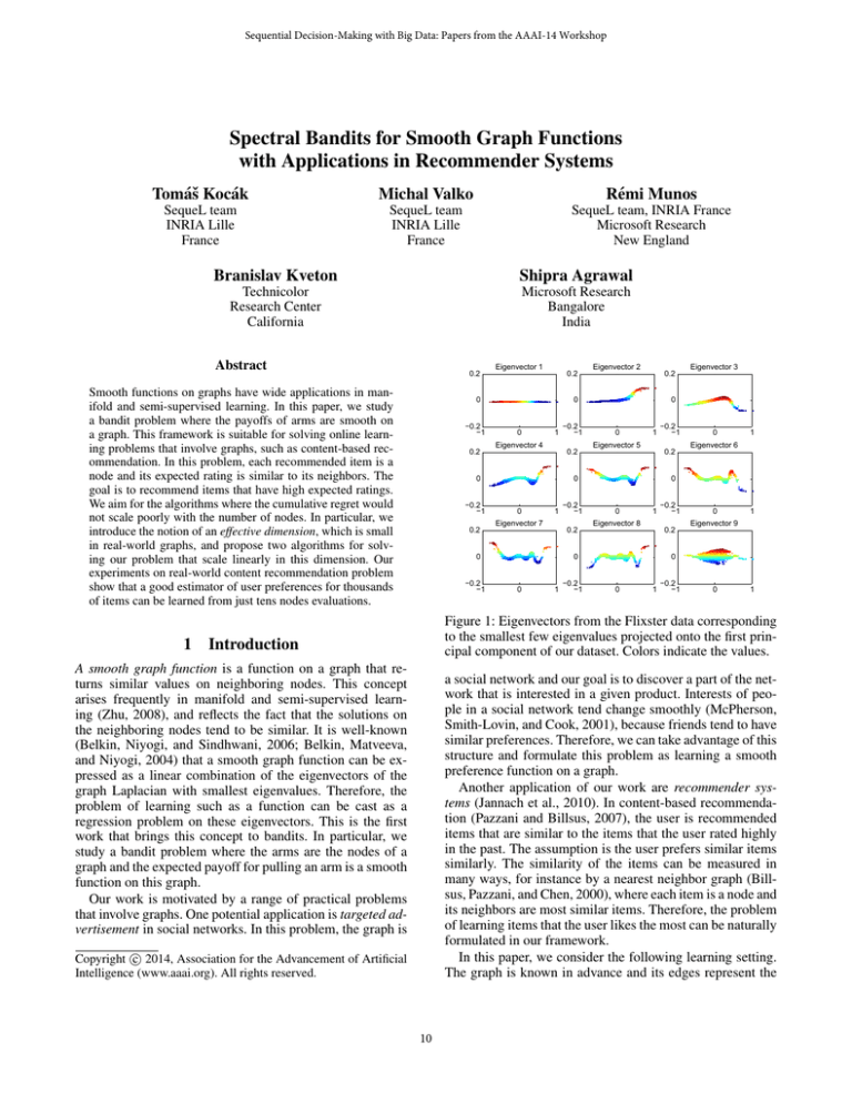
Figure 1: Eigenvectors from the Flixster data corresponding
to the smallest few eigenvalues projected onto the first principal component of our dataset. Colors indicate the values.
Introduction
A smooth graph function is a function on a graph that returns similar values on neighboring nodes. This concept
arises frequently in manifold and semi-supervised learning (Zhu, 2008), and reflects the fact that the solutions on
the neighboring nodes tend to be similar. It is well-known
(Belkin, Niyogi, and Sindhwani, 2006; Belkin, Matveeva,
and Niyogi, 2004) that a smooth graph function can be expressed as a linear combination of the eigenvectors of the
graph Laplacian with smallest eigenvalues. Therefore, the
problem of learning such as a function can be cast as a
regression problem on these eigenvectors. This is the first
work that brings this concept to bandits. In particular, we
study a bandit problem where the arms are the nodes of a
graph and the expected payoff for pulling an arm is a smooth
function on this graph.
Our work is motivated by a range of practical problems
that involve graphs. One potential application is targeted advertisement in social networks. In this problem, the graph is
a social network and our goal is to discover a part of the network that is interested in a given product. Interests of people in a social network tend change smoothly (McPherson,
Smith-Lovin, and Cook, 2001), because friends tend to have
similar preferences. Therefore, we can take advantage of this
structure and formulate this problem as learning a smooth
preference function on a graph.
Another application of our work are recommender systems (Jannach et al., 2010). In content-based recommendation (Pazzani and Billsus, 2007), the user is recommended
items that are similar to the items that the user rated highly
in the past. The assumption is the user prefers similar items
similarly. The similarity of the items can be measured in
many ways, for instance by a nearest neighbor graph (Billsus, Pazzani, and Chen, 2000), where each item is a node and
its neighbors are most similar items. Therefore, the problem
of learning items that the user likes the most can be naturally
formulated in our framework.
In this paper, we consider the following learning setting.
The graph is known in advance and its edges represent the
c 2014, Association for the Advancement of Artificial
Copyright Intelligence (www.aaai.org). All rights reserved.
10
want to assume such an extreme case (i.e. αi∗ = 0 for i > k).
Therefore, we opt for the more plausible assumption that the
coefficients with the high indexes are small. Consequently,
we deliver algorithms with the performance that scale with
the norm of α∗ which expresses smoothness with respect to
the graph.
The learning setting is the following. In each time step
t ≤ T , the recommender π chooses a node π(t) and obtains
a noisy reward rt = xTπ(t) α∗ + εt , where the noise εt is
assumed to be R-sub-Gaussian for any t, i.e.,
2 2
ξ R
ξεt
N
∀ξ ∈ R, E[e | {bi }i=1 , Ht−1 ] ≤ exp
.
2
similarity of the nodes in the graph. At time t, we choose
a node and then observe its payoff. In targeted advertisement, this may correspond to showing an ad and then observing whether the person clicked on the ad. In contentbased recommendation, this may correspond to recommending an item and then observing the assigned rating. Based on
the payoff, we update our model of the world and then the
game proceeds into time t + 1. Since the number of nodes N
can be huge, we are interested in the regime when t < N .
If the smooth graph function can be expressed as a linear combination of k eigenvectors of the graph Laplacian,
and k is small and known, our learning problem can be
solved trivially using ordinary linear bandits (Auer, 2002;
Li et al., 2010). In practice, k is problem specific and unknown. Moreover, the number of features k may approach
the number of nodes N . Therefore, proper regularization is
necessary so that the regret of the learning algorithm does
not scale with N . We are interested in the setting where the
regret is independent of N and therefore our problem is nontrivial.
We make several major contributions. First, we formalize
a bandit problem, where the payoff of the arms is a smooth
function on a graph. Second, we propose
for
√ two algorithms
√
solving this problem that achieve d T ln T and d T ln N
expected cumulative regret, where d is the effective dimension of the problem. Finally, we evaluate both of the algorithms on synthetic and real-world content-based recommendation problems.
2
In our setting we have xv ∈ RD and kxv k2 ≤ 1 for all xv .
The goal of the recommender is to minimize the cumulative
regret with respect to the strategy that always picks the best
node w.r.t. α∗ . Let π(t) be the node picked (referred to as
pulling an arm) by an algorithm π at time t. The cumulative
(pseudo) regret of π is defined as:
RT = T max fα∗ (v) −
v
fα (v) =
fα∗ (π(t)).
t=1
We call this bandit setting spectral since it is built on the
spectral properties of a graph. Compared to the linear and
multi-arm bandits, the number of arms K is equal to the
number of nodes N and also to the dimension of the basis D
(each eigenvector is of dimension N ). However, a regret that
scales with N or D that can be obtained using those settings
is not acceptable because the number of nodes can be large.
While we are mostly interested in the setting with K = N ,
our algorithms and analyses can be applied for any finite K.
Setting
Let G be the given graph with the set of nodes V and denote
|V| = N the number of nodes. Let W be the N × N matrix of similarities wij (edge weights) and
P D is the N × N
diagonal matrix with the entries dii = j wij . The graph
N
Laplacian of G is defined as L = D − W. Let {λL
k , qk }k=1
be the eigenvalues and eigenvectors of L ordered such that
T
L
L
0 = λL
1 ≤ λ2 ≤ · · · ≤ λN . Equivalently, let L = QΛL Q
be the eigendecomposition of L, where Q is an N × N orthogonal matrix with eigenvectors in columns.
In our setting we assume that the reward function is a linear combination of the eigenvectors. For any set of weights
α let fα : V → R be the function linear in the basis of the
eigenvectors of L:
N
X
T
X
3
Effective dimension
In order to present our algorithms and analyses we introduce
a notion of effective dimension d. We keep using capital D
to denote the ambient dimension, which is equal to N in the
spectral bandits setting. Intuitively, the effective dimension
is a proxy for number of relevant dimensions. We first provide a formal definition and then discuss its properties.
In general, we assume there exists a diagonal matrix Λ
with the entries 0 < λ = λ1 ≤ λ2 ≤ · · · ≤ λN and a
set of K vectors x1 , . . . , xK ∈ RN such that kxi k2 ≤ 1
for all i. For the smooth graph functions, we have K = N .
Moreover since Q is an orthonormal matrix, kxi k2 = 1.
Finally, since the first eigenvalues of a graph Laplacian is
always zero, λL
1 = 0, we use Λ = ΛL + λI, in order to have
λ1 = λ.
Definition 1. Let the effective dimension d be the largest d
such that:
T
(d − 1)λd ≤
log(1 + T /λ)
The effective dimension d is small when the coefficients
λi grow rapidly above T . This is the case when the dimension of the space D (and K) are much larger than T , such
as in graphs from social networks with very large number
of nodes N . In the contrary, when the coefficients are all
small then d may be of order T which would make the regret
αk (qk )v = hxv , αi,
k=1
where xv is the v-th row of Q, i.e., (xv )i = (qi )v . If
the weight coefficients of the true α∗ are such that the
large coefficients correspond to the eigenvectors with the
small eigenvalues and vice versa, then fα∗ would be a
smooth function on G (Belkin, Niyogi, and Sindhwani,
2006). Figure 1 displays first few eigenvectors of the Laplacian constructed from data we use in our experiments.
In the extreme case, the true α∗ may be of the form
[α1∗ , α2∗ , . . . , αk∗ , 0, 0, 0]TN for some k N . Had we known
k in such case, the known linear bandits algorithm would
work with the performance scaling with k instead of D. Unfortunately, first, we do not know k and second, we do not
11
Algorithm 1 SpectralUCB
Input:
N : the number of vertices, T : the number of pulls
{ΛL , Q} spectral basis of L
λ, δ : regularization and confidence parameters
R, C : upper bounds on the noise and kα∗ kΛ
Run:
Λ ← ΛL + λI
d ← max{d : (d − 1)λd ≤ T / log(1 + T /λ)}
for t = 1 to T do
Update basis coefficients α̂:
Xt ← [x1 , . . . , xt−1 ]T
r ← [r1 , . . . , rt−1 ]T
Vt ← Xt XTt + Λ
α̂t ← p
Vt−1 XTt r
ct ← 2R d log(1 + t/λ) + 2 log(1/δ) + C
Choose node vt (x
vt -th row of Q)
vt ← arg maxv fα̂ (v) + ct kxv kV−1
t
Observe reward rt
end for
advantage of our analysis to define ct based on the effective
dimension d which is specifically tailored to our setting. The
following theorem characterizes the performance of SpectralUCB and bounds the regret as a function of effective dimension d.
Theorem 1 (Valko et al. (2014)). Let d be the effective dimension and λ be the minimum eigenvalue of Λ. If kα∗ kΛ ≤
C and for all xv , hxv , α∗ i ∈ [−1, 1], then the cumulative regret of SpectralUCB is with probability at least 1 − δ
bounded as:
h p
i
RT ≤ 8R d log(1 + T /λ) + 2 log(1/δ) + 4C + 4
p
× dT log(1 + T /λ)
Remark 1. The constant C needs to be such that kα∗ kΛ ≤
C. If we set C too small, the true α∗ will lie outside of the
region and far from α̂t , causing the algorithm to underperform. Alternatively C can time dependent, e.g. Ct = log T .
In such case we do not need to know an upperbound on
kα∗ kΛ in advance, but our regret bound would only hold
after some t, where Ct ≥ kα∗ kΛ .
Spectral Thompson Sampling
bounds useless. Figure 2 shows how d behaves compared to
D on the generated and the real Flixster network graphs1
that we use for the experiments.
In this section, we use the Thompson Sampling approach
to decide which arm to play. Specifically, we will represent
our current knowledge about α∗ as the normal distribution
N (α̂(t), v 2 Vt−1 ), where α̂(t) is our actual approximation
of the unknown parameter α∗ and v 2 Vt−1 reflects of our uncertainty about it for some constant v specificaly selected
using your analysis (Kocák et al. (2014)). As mentioned before, we assume that the reward function is a linear combination of eigenvectors of L with large coefficients corresponding to the eigenvectors with small eigenvalues. We encode this assumption into our initial confidence ellipsoid by
setting V1 = Λ = ΛL + λI, where λ is a regularization
parameter.
After that, every time step t we generate a sample α̃(t)
from distribution N (α̂(t), v 2 Vt−1 ) and chose an arm π(t),
that maximizes xTi α̃(t). After receiving a reward, we update
our estimate of α∗ and the confidence of it, i.e. we compute
α̂(t + 1) and V(t + 1),
Flixster graph: N=4546
Barabasi−Albert graph N=500
11
7
10
9
effective dimenstion
effective dimenstion
6
5
4
3
8
7
6
5
4
3
2
2
1
1
0
50
100
150
200
250
300
350
400
450
500
500
1000
time T
1500
2000
2500
3000
3500
4000
4500
time T
Figure 2: Effective dimension d in the regime T < N . The
effective dimension for this data is much smaller than the
ambient dimension D, which is 500 and 4546 respectively.
4
Algorithms
In this section we propose two algorithms. The first algorithm is based on LinUCB. For the second algorithm we use
Thompson sampling approach.
Vt+1 = Vt + xπ(t) xTπ(t)
α̂(t + 1) =
SpectralUCB
t
X
!
xπ(i) r(i) .
i=1
The first algorithm we present is SpectralUCB (Algorithm 1)
which is based on LinUCB and uses the spectral penalty.
For clarity, we set xt = xvt = xπ(t) . Here we consider
regularized least-squares estimate α̂t of the form:
!
t
X
2
α̂t = arg min
[hxτ , αi − rτ ] + kαkΛ .
α
−1
Vt+1
The computational advantage of SpectralTS in Algorithm 2, compared to SpectralUCB, is that we do not need
to compute the confidence bound for each arm. Indeed, in
SpectralTS we need to sample α̃ which can be done in N 2
time (note that Vt is only changing by a rank one update)
and a maximum of xTi α̃ which can be also done in N 2 time.
On the other hand, in SpectralUCB, we need to compute a
Vt−1 norm for each of N context vectors which amounts to
a N D2 time. Table 1 (left) summarizes the computational
complexity of the two approaches. Finally note that in our
setting D = N , which comes to a N 2 vs. N 3 time per step.
We support this argument in Section 5. Finally note that the
τ =1
A key part of the algorithm is to define the ct kxkV−1 cont
fidence widths for the prediction of the rewards. We take
1
We set Λ to ΛL + λI with λ = 0.01, where ΛL is the graph
Laplacian of the respective graph.
12
Optimistic Approach
D 2 N per step update
Thompson Sampling
D 2 + DN per step update
Linear
Spectral
LinUCB
√
SpectralUCB
√
LinearTS
√
SpectralTS
√
D T ln T
D T ln N
Remark 2. Substituting
g and p we see that regret bound
√
scales with d T ln N . Note that N = D could
√ be exponential in d and we need to consider factor ln N in our
bound. On the other hand if√N is exponential in d,
√then our
algorithm scales with ln D T ln D = ln(D)3/2 T which
is even better.
d T ln T
d T ln N
Table 1: Linear vs. Spectral Bandits
5
eigendecomposition needs to be done only once in the beginning and since L is diagonally dominant, this can be done
for N in millions (Koutis, Miller, and Peng, 2010).
Experiments
The aim of this section is to give empirical evidence that
SpectralTS and SpectralUCB deliver better empirical performance than LinearTS and LinUcb in T < N regime. For
the synthetic experiment, we considered a Barabási-Albert
(BA) model (1999), known for its preferential attachment
property, common in real-world graphs. We generated a random graph using BA model with N = 250 nodes and the
degree parameter 3. For each run, we generated the weights
of the edges uniformly at random. Then we generated α∗ , a
random vector of weights (unknown) to algorithms in order
to compute the payoffs and evaluated the cumulative regret.
The α∗ in each simulation was a random linear combination
of the first 3 smoothest eigenvectors of the graph Laplacian.
In all experiments, we had δ = 0.001, λ = 1, and R = 0.01.
We evaluated the algorithms in T < N regime, where the
linear bandit algorithms are not expected to perform well.
Figure 3 shows the results averaged over 10 simulations.
Notice that while the result of SpectralTS are comparable
to SpectralUCB, its computational time is much faster due
the reasons discussed in Section 4. Recall that while both algorithms compute the least-square problem of the same size,
SpectralUCB has then to compute the confidence interval for
each arm.
Algorithm 2 Spectral Thompson Sampling
Input:
N : number of arms, T : number of pulls
{ΛL , Q}: spectral basis of graph Laplacian L
λ, δ: regularization and confidence parameters
R, C: upper bounds on noise and kα∗ kΛ
Initialization:
p
v = R 6d ln((λ + T )/δλ) + C
α̂ = 0N , f = 0N , V = ΛL + λIN
Run:
for t = 1 to T do
Sample α̃ ∼ N (α̂, v 2 V−1 )
π(t) ← arg maxa xTa α̃
Observe a noisy reward r(t) = xTπ(t) α∗ + ε
f ← f + xπ(t) r(t)
Update V ← V + xπ(t) xTπ(t)
Update α̂ ← V−1 f
end for
We would like to stress that we consider the regime when
T < N , because we aim for applications with a large set
of arms and we are interested in a satisfactory performance
after just a few iterations. For instance, when we aim to recommend N movies, we would like to have useful recommendations in the time T < N , i.e., before the user saw all
of them. The following theorem upperbounds the cumulative
regret of SpectralTS in terms of d.
Theorem 2 (Kocák et al. (2014)). Let d be the effective dimension and λ be the minimum eigenvalue of Λ. If kα∗ kΛ ≤
C and for all xi , |xTi α∗ | ≤ 1, then the cumulative regret
of Spectral Thompson Sampling is with probability at least
1 − δ bounded as
r
λ+T
1
11g 4 + 4λ
dT ln
+
RT ≤
p
λ
λ
T
r
g 11
2
√ +2
+
2T ln ,
p
δ
λ
√
where p = 1/(4e π) and
s
!
√
λ+T
g = 4 ln T N R 6d ln
+C
δλ
s
(λ + T )T 2
+ R 2d ln
+ C.
δλ
Barabasi−Albert N=250, basis size=3, effective d=1
5
45
SpectralTS
40
LinearTS
SpectralUCB
LinUCB
35
30
computational time in seconds
cumulative regret
50
25
20
15
10
5
0
0
4
3
2
1
0
40
80
time T
120
160
200
SpectralTS
LinearTS
SpectralUCB
LinUCB
Figure 3: Barabási-Albert random graph results
Furthermore, we performed the comparison MovieLens
dataset (Lam and Herlocker, 2012) of the movie ratings. The
graph in this dataset is the graph of 2019 movies edges corresponding to the movie similarities. We completed the missing ratings by a low-rank matrix factorization and used it
construct a 10-NN similarity graph. For each user we have
a graph function, unknown to the algorithms, that assigns to
each node, the rating of the particular user. A detailed description on the preprocessing is deferred to (Valko et al.,
2014) due to the limited space. Our goal is then to recommend the most highly rated content. Figure 4 shows the
MovieLens data results averaged over 10 randomly sampled
users. Notice that the results follow the same trends as for
synthetic data.
13
Movielens data N=2019, average of 10 users, T=200, d = 5
2500
cumulative regret
250
200
computational time in seconds
300
SpectralUCB
LinUCB
SpectralTS
LinearTS
150
100
50
0
0
2000
1500
1000
500
0
40
80
time t
120
160
200
SpectralTS
LinearTS SpectralUCB
LinUCB
Figure 4: MovieLens data results
References
Auer, P. 2002. Using confidence bounds for exploitationexploration trade-offs. Journal of Machine Learning Research 3:397–422.
Barabasi, A.-L., and Albert, R. 1999. Emergence of scaling
in random networks. Science 286:11.
Belkin, M.; Matveeva, I.; and Niyogi, P. 2004. Regularization and Semi-Supervised Learning on Large Graphs. In
Conference on Learning Theory.
Belkin, M.; Niyogi, P.; and Sindhwani, V. 2006. Manifold Regularization: A Geometric Framework for Learning
from Labeled and Unlabeled Examples. Journal of Machine
Learning Research 7:2399–2434.
Billsus, D.; Pazzani, M. J.; and Chen, J. 2000. A learning
agent for wireless news access. In IUI, 33–36.
Jannach, D.; Zanker, M.; Felfernig, A.; and Friedrich, G.
2010. Recommender Systems: An Introduction. Cambridge
University Press.
Kocák, T.; Valko, M.; Munos, R.; and Agrawal, S. 2014.
Spectral Thompson Sampling. In Proceedings of the
Twenty-Eighth AAAI Conference on Artificial Intelligence.
Koutis, I.; Miller, G. L.; and Peng, R. 2010. Approaching Optimality for Solving SDD Linear Systems. In 2010
IEEE 51st Annual Symposium on Foundations of Computer
Science, 235–244. IEEE.
Lam, S., and Herlocker, J. 2012. MovieLens 1M Dataset.
http://www.grouplens.org/node/12.
Li, L.; Chu, W.; Langford, J.; and Schapire, R. E. 2010. A
Contextual-Bandit Approach to Personalized News Article
Recommendation. WWW 10.
McPherson, M.; Smith-Lovin, L.; and Cook, J. 2001. Birds
of a Feather: Homophily in Social Networks. Annual Review
of Sociology 27:415–444.
Pazzani, M. J., and Billsus, D. 2007. Content-Based Recommendation Systems. The adaptive web.
Valko, M.; Munos, R.; Kveton, B.; and Kocák, T. 2014.
Spectral Bandits for Smooth Graph Functions. In 31th International Conference on Machine Learning.
Zhu, X. 2008. Semi-Supervised Learning Literature Survey.
Technical Report 1530, University of Wisconsin-Madison.
14