Proceedings of the Twenty-Ninth AAAI Conference on Artificial Intelligence
Learning to Hash on Structured Data
Qifan Wang, Luo Si and Bin Shen
Computer Science Department, Purdue University
West Lafayette, IN 47907, US
wang868@purdue.edu, lsi@purdue.edu, bshen@purdue.edu
Abstract
Hashing techniques have been widely applied for large scale
similarity search problems due to the computational and
memory efficiency. However, most existing hashing methods assume data examples are independently and identically
distributed. But there often exists various additional dependency/structure information between data examples in many
real world applications. Ignoring this structure information
may limit the performance of existing hashing algorithms.
This paper explores the research problem of learning to Hash
on Structured Data (HSD) and formulates a novel framework
that considers additional structure information. In particular,
the hashing function is learned in a unified learning framework by simultaneously ensuring the structural consistency
and preserving the similarities between data examples. An
iterative gradient descent algorithm is designed as the optimization procedure. Furthermore, we improve the effectiveness of hashing function through orthogonal transformation
by minimizing the quantization error. Experimental results on
two datasets clearly demonstrate the advantages of the proposed method over several state-of-the-art hashing methods.
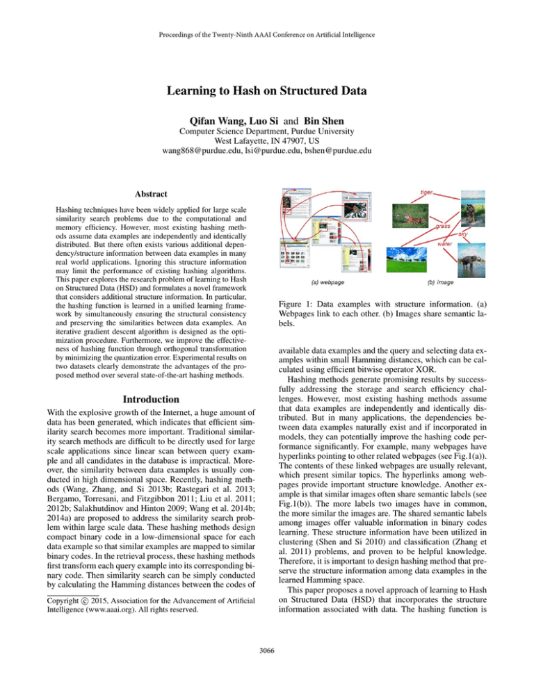
Figure 1: Data examples with structure information. (a)
Webpages link to each other. (b) Images share semantic labels.
available data examples and the query and selecting data examples within small Hamming distances, which can be calculated using efficient bitwise operator XOR.
Hashing methods generate promising results by successfully addressing the storage and search efficiency challenges. However, most existing hashing methods assume
that data examples are independently and identically distributed. But in many applications, the dependencies between data examples naturally exist and if incorporated in
models, they can potentially improve the hashing code performance significantly. For example, many webpages have
hyperlinks pointing to other related webpages (see Fig.1(a)).
The contents of these linked webpages are usually relevant,
which present similar topics. The hyperlinks among webpages provide important structure knowledge. Another example is that similar images often share semantic labels (see
Fig.1(b)). The more labels two images have in common,
the more similar the images are. The shared semantic labels
among images offer valuable information in binary codes
learning. These structure information have been utilized in
clustering (Shen and Si 2010) and classification (Zhang et
al. 2011) problems, and proven to be helpful knowledge.
Therefore, it is important to design hashing method that preserve the structure information among data examples in the
learned Hamming space.
This paper proposes a novel approach of learning to Hash
on Structured Data (HSD) that incorporates the structure
information associated with data. The hashing function is
Introduction
With the explosive growth of the Internet, a huge amount of
data has been generated, which indicates that efficient similarity search becomes more important. Traditional similarity search methods are difficult to be directly used for large
scale applications since linear scan between query example and all candidates in the database is impractical. Moreover, the similarity between data examples is usually conducted in high dimensional space. Recently, hashing methods (Wang, Zhang, and Si 2013b; Rastegari et al. 2013;
Bergamo, Torresani, and Fitzgibbon 2011; Liu et al. 2011;
2012b; Salakhutdinov and Hinton 2009; Wang et al. 2014b;
2014a) are proposed to address the similarity search problem within large scale data. These hashing methods design
compact binary code in a low-dimensional space for each
data example so that similar examples are mapped to similar
binary codes. In the retrieval process, these hashing methods
first transform each query example into its corresponding binary code. Then similarity search can be simply conducted
by calculating the Hamming distances between the codes of
c 2015, Association for the Advancement of Artificial
Copyright Intelligence (www.aaai.org). All rights reserved.
3066
to obtain more effective hashing codes via a matrix factorization formulation. More recently, some multi-view hashing methods (Gong et al. 2014; Zhang, Wang, and Si 2011;
Ding, Guo, and Zhou 2014) have been proposed to deal with
multi-modal data for cross-view similarity search. These
multi-view methods can be applied by treating the structure
information as second view. However, structure information
is usually very sparse, e.g., each webpage may contain very
few hyperlinks. Directly using it as a second information
source can lead to unreliable results. More discussion will
be provided later in the experiments.
learned in a unified learning framework by simultaneously
ensuring the structural consistency and preserving the similarities between data examples. In particular, the objective
function of the proposed HSD approach is composed of
two parts: (1) Structure consistency term, which ensures the
hashing codes to be consistent with the structure information. (2) Similarity preservation term, which aims at preserving the similarity between data examples in the learned
hashing codes. An iterative gradient descent algorithm is designed as the optimization procedure. We further improve
the quality of hashing function by minimizing the quantization error. Experimental results on two datasets demonstrate
the superior performance of the proposed method over several state-of-the-art hashing methods.
The rest of this paper is organized as follows. Section 2
reviews previous hashing methods. Section 3 presents the
formulation of the proposed HSD hashing method. Section
4 describes the optimization method together with the orthogonal transformation. Some analysis of the algorithm is
also provided. The experimental results and discussions are
given in Section 5. Section 6 concludes and points out some
future directions.
Hashing on Structured Data
Problem Setting
Before presenting the details, we first introduce some notations. Assume there are total n training examples. Let us
denote their features as: X = {x1 , x2 , . . . , xn } ∈ Rd×n ,
where d is the dimensionality of the feature. A directed or
undirected graph G = (V, E) is used to depict the structure between data examples. Each node v ∈ V corresponds
to a data example, and an edge e = (i, j) ∈ E with a
weight wij represents a link/connection between nodes i and
j. The larger the weight wij is, the more relevant xi and xj
should be. We will discuss how to assign w later. The goal
is to obtain a linear hashing function f : Rd → {−1, 1}k ,
which maps data examples X to their binary hashing codes
Y = {y1 , y2 , . . . , yn } ∈ {−1, 1}k×n (k is the length of
hashing code). The linear hashing function is defined as:
Related Work
Locality-Sensitive Hashing (LSH) (Datar et al. 2004) is
one of the most commonly used data-independent hashing methods. It utilizes random linear projections, which
are independent of training data, to map data points from
a high-dimensional feature space to a low-dimensional binary space. This method has been extended to Kernelized
Locality-Sensitive Hashing (Raginsky and Lazebnik 2009;
Kulis and Grauman 2009) by exploiting kernel similarity for
better retrieval efficacy. Another class of hashing methods
are called data-dependent methods, whose projection functions are learned from training data. These data-dependent
methods include spectral hashing (SH) (Weiss, Torralba, and
Fergus 2008), principal component analysis based hashing
(PCAH) (Lin, Ross, and Yagnik 2010), self-taught hashing
(STH) (Zhang et al. 2010) and iterative quantization (ITQ)
(Gong et al. 2012). SH learns the hashing codes based on
spectral graph partitioning and forcing the balanced and uncorrelated constraints into the learned codes. PCAH utilizes
principal component analysis (PCA) to learn the projection
functions. STH combines an unsupervised learning step with
a supervised learning step to learn effective hashing codes.
ITQ learns an orthogonal rotation matrix to refine the initial projection matrix learned by PCA so that the quantization error of mapping the data to binary codes is minimized.
Compared with the data-independent methods, these datadependent methods generally provide more effective hashing codes.
Recently, supervised hashing methods (Liu et al. 2012a;
Wang, Zhang, and Si 2013a; Wang et al. 2013; Wang, Si, and
Zhang 2014; Wang et al. 2014c) have incorporated labeled
data/information, e.g. semantic tags, for learning more effective hashing function. For example, in semi-supervised hashing (Wang, Kumar, and Chang 2012) method, pairwise similarity constraints are imposed in the learning framework.
In work (Wang, Si, and Zhang 2014), tags are incorporated
H T xi )
yi = f (xi ) = sgn(H
(1)
where H ∈ Rd×k is the coefficient matrix representing the
hashing function and sgn is the sign function. yi ∈ {−1, 1}k
is the binary hashing code1 of xi .
The objective function of HSD is composed of two components: (1) Structure consistency, which ensures that the
hashing codes are consistent with the structure information.
(2) Similarity preservation, which aims at preserving the
data similarity in the learned hashing codes. In the rest of
this section, we will present the formulation of these two
components respectively. Then we will describe the optimization algorithm together with a scheme that can further
improve the quality of the hashing function by minimizing
the quantization error.
Structure Consistency
Our motivation is that the similarity between the learned
hashing codes should agree or be consistent with the structure information defined on the graph G. Specifically, a pair
of nodes linked by an edge tend to have similar hashing
codes. The larger the weight between nodes i and j, the
smaller the Hamming distance between their codes should
be. For webpages, we define the weight wij associated with
edge (i, j) to be the number of hyperlinks between the two
webpages. Similarly for images, we assign weight wij using
the number of common labels shared by image xi and xj .
1
We generate hashing bits as {−1, 1}, which can be simply
converted to {0, 1} valued hashing codes.
3067
Overall Objective
Then a structure consistency component can be directly
formulated as:
X
1 X
wij dH (yi , yj ) =
wij kyi − yj k2
(2)
4
(i,j)∈E
The entire objective function consists of three components:
the structure consistency term in Eqn.3, the similarity preservation term given in Eqn.6 and an orthogonal constraint term
as follows:
H T X )W̄ sgn(X
XTH)
min tr sgn(H
H
H T X )S̄
X T H ) + β kH
H T H − I k2F
+α tr sgn(H
S̄sgn(X
(7)
where α and β are trade-off parameters to balance the
weights among the terms. The orthogonality constraint enforce the hashing bits to be uncorrelated with each other and
therefore the learned hashing codes can hold least redundant
information.
(i,j)∈E
dH (yi , yj )= 14 kyi − yj k2
binary codes yi and yj .
where
is the Hamming distance between
This definition says that for
each linked node pair (i, j), the Hamming distance between
the corresponding hashing codes yi and yj should be consistent with the edge weight wij . In other words, we assign
a heavy penalty if two strongly connected data examples are
mapped far away.
By substituting Eqn.1 with some additional mathematical
operations, the above equation can be rewritten as a compact
matrix form as:
Y T = tr sgn(H
H T X )W̄ sgn(X
XTH)
(3)
tr Y W̄
W̄Y
Optimization Algorithm
Relaxation
where tr() is the matrix trace function. W̄ = D − W is
called graph Laplacian (Weiss, Torralba, and Fergus 2008)
and D isPa diagonal n × n matrix whose entries are given by
n
D ii = j=1 wij . By minimizing the structure consistency
term, structure information is well preserved in Hamming
space by hashing function H .
Directly minimizing the objective function in Eqn.7 is intractable since it is an integer programming problem, which
is proven to be NP-hard to solve. Therefore, we use the
signed magnitude instead of the sign function as suggested
in (Wang et al. 2013; Wang, Si, and Zhang 2014). Then the
relaxed objective function becomes:
min tr H̃ T LH̃ + β kH̃ T H̃ − I k2F
(8)
Similarity Preservation
One of the key problems in hashing algorithms is similarity preserving, which indicates that similar data examples
should be mapped to similar hashing codes within a short
Hamming distance. To measure the similarity between data
examples represented by the binary hashing codes, one natural way is to minimize the weighted average Hamming distance as follows:
X
S ij kyi − yj k2
(4)
H̃
X T and can be pre-computed. H̃
S̄)X
where L ≡ X (W̄ + αS̄)
represents the relaxed solution. Although the relaxed objective in Eqn.8 is still non-convex, it is smooth and differentiable which enables gradient descent methods to be applied
for efficient optimization. The gradients of the two terms
with respect to H̃ are given below:
d Eqn.8
LH̃ + 4βH̃
(9)
H̃(H̃ T H̃ − I )
= 2L
d H̃
With this obtained gradient, L-BFGS quasi-Newton method
(Liu and Nocedal 1989) is applied to solve the optimization
problem.
i,j
Here, Sij is the pairwise similarity between data example xi
and xj . To meet the similarity preservation criterion, we seek
to minimize this quantity, because it incurs a heavy penalty
if two similar examples have very different hashing codes.
There are many different ways of defining the similarity
matrix S . In SH (Weiss, Torralba, and Fergus 2008), the authors used the global similarity structure of all data pairs,
while in (Zhang, Wang, and Si 2011), the local similarity
structure, i.e., k-nearest-neighborhood, is used. In this paper, we use the local similarity, due to its nice property in
many machine learning applications. In particular, the corresponding weights are computed by Gaussian functions:

2
jk
 − kxiσ−x
2
ij
, if xi ∈ Nk (xj ) or xj ∈ Nk (xi )
S ij = e

0,
otherwise
(5)
The variance σij is determined automatically by local scaling (Zelnik-Manor and Perona 2004), and Nk (x) represents
the set of k-nearest-neighbors of data example x. Similarly,
Eqn.4 can be rewritten as a compact form:
Y T = tr sgn(H
H T X )S̄
XTH)
tr Y S̄
S̄Y
S̄sgn(X
(6)
By minimizing this term, the similarity between different
data examples can be preserved in the learned hashing codes.
Orthogonal Transformation
After obtaining the optimal hashing function H̃ from the relaxation, the hashing codes Y can be generated using Eqn.1.
It is obvious that the quantization error can be measured as
Y − H̃ T X k2F . Inspired by (Gong et al. 2012), we propose
kY
to further improve the hashing function by minimizing this
quantization error using an orthogonal transformation. We
first prove the following orthogonal invariant theorem.
Theorem 1. Assume Q is a k × k orthogonal matrix, i.e.,
Q T Q = I . If H̃ is an optimal solution to the relaxed problem
in Eqn.8, then H̃Q is also an optimal solution.
Proof.
H̃Q
By substituting
into Eqn.8, we
have:
T
T
T
tr (H̃Q
H̃Q) LH̃Q = tr Q H̃ LH̃Q = tr H̃ T LH̃ ,
QT (H̃ T H̃ − I )Q
Qk2F =
and k(H̃Q
H̃Q)T H̃Q − I k2F = kQ
kH̃ T H̃ − I k2F .
Thus, the value of the objective function in Eqn.8 does not
change by the orthogonal transformation.
3068
Algorithm 1 Hashing on Structured Data (HSD)
Input: Data examples X , Structure graph G and trade-off
parameters
Output: Hashing function H and Hashing codes Y
Initialize H and Q = I , Calculate L .
repeat
Compute the gradient in Eqn.9 and update H̃
until the solution converges
repeat
Update Y using Eqn.11
Update Q = V S T according to Theorem 2.
until the solution converges
Compute hashing function H =H̃Q
H̃Q.
According to the above theorem, we propose to find a better hashing function H = H̃Q by minimizing the quantization error between the binary hashing codes and the orthogonal transformation of the relaxed solution as follows:
Y − (H̃Q
min kY
H̃Q)T X k2F
Y,Q
s.t.
(10)
Y ∈ {−1, 1}k×n , QT Q = I
Intuitively, we seek binary codes that are close to some
orthogonal transformation of the relaxed solution. The orthogonal transformation not only preserves the optimality
of the relaxed solution but also provides us more flexibility to achieve better hashing codes with low quantization error. The idea of orthogonal transformation is also utilized in
ITQ (Gong et al. 2012). However, ITQ method is not designed for incorporating structure information into learning
effective hashing function and it does not preserve the local
similarities among data examples. The above optimization
problem can be solved by minimizing Eqn.10 with respect
to Y and Q alternatively as follows:
Fix Q and update Y . The closed form solution can be
expressed as:
HTX)
H̃Q)T X = sgn(H
(11)
Y = sgn (H̃Q
Experimental Results
Datasets and Setting
We evaluate our method on two datasets: W ebKB and
NUS-WIDE. W ebKB 2 contains 8280 webpages in total
collected from four universities. The webpages without any
incoming and outgoing links are deleted, resulting in a subset of 6883 webpages. The tf-idf (normalized term frequency
and log inverse document frequency) (Manning, Raghavan,
and Schütze 2008) features are extracted for each webpage.
90% documents (6195) are randomly selected as training
data, while the remaining (688) documents are used for testing. NUS-WIDE 3 (Chua et al. 2009) is created by NUS lab
for evaluating image annotation and retrieval techniques. It
contains 270k images associated with 81 ground truth labels. A subset of 21k images associated with these semantic labels are used in our experiments. 500-dimensional visual features are extracted using a bag-of-visual-word model
with local SIFT descriptor (Lowe 2004). We randomly partition this dataset into two parts, 1k for testing and 20k for
training.
We implement our algorithm using Matlab on a PC with
Intel Duo Core i5-2400 CPU 3.1GHz and 8GB RAM. The
parameter α and β are tuned by 5-fold cross validation
through the grid {0.01, 0.1, 1, 10, 100} on the training set
and we will discuss more details on how it affects the performance of our approach later. We repeat each experiment
10 times and report the result based on the average over these
runs. Each run adopts a random split of the dataset.
which is identical with our linear hashing function in Eqn.1.
Fix Y and update Q. The objective function becomes:
Y − Q T H̃ T X k2F
min kY
Q T Q =II
(12)
In this case, the objective function is essentially the classic
Orthogonal Procrustes problem (Schonemann 1966), which
can be solved efficiently by singular value decomposition
using the following theorem (we refer to (Schonemann
1966) for the detailed proof).
Theorem 2. Let SΛV T be the singular value decomposiH̃. Then Q = V S T minimizes the objective
tion of Y X T H̃
function in Eqn.12.
We then perform the above two steps alternatively to obtain the optimal hashing codes and the orthogonal transform
matrix. In our experiments, we find that the algorithm usually converges in about 40∼60 iterations. The full learning
algorithm is described in Algorithm 1.
Complexity Analysis
This section provides some analysis on the training cost of
the optimization algorithm. The optimization algorithm of
HSD consists of two main loops. In the first loop, we iteratively solve for H̃ to obtain the relaxed solution, where the
time complexities for computing the gradient in Eqn.9 are
bounded by O(nkd + nk 2 ). The second loop iteratively optimizes the binary hashing codes and the orthogonal transformation matrix, where the time complexities for updating
Y and Q are bounded by O(nk 2 + nkd + k 3 ). Moreover,
both two loops take less than 60 iterations to converge in our
experiments. Thus, the total time complexity of the learning
algorithm is bounded by O(nkd + nk 2 + k 3 ), which scales
linearly with n given n d > k. For each query, the hashing time is constant O(dk).
Comparison Methods
The proposed Hashing on Structure Data (HSD) approach
is compared with five different hashing methods, including Locality Sensitivity Hashing (LSH) (Datar et al. 2004),
Spectral Hashing (SH) (Weiss, Torralba, and Fergus 2008),
ITerative Quantization (ITQ) (Gong et al. 2012), Composite Hashing from Multiple Information Sources (CHMIS)
(Zhang, Wang, and Si 2011) and Collective Matrix Factorization Hashing (CMFH) (Ding, Guo, and Zhou 2014). LSH,
SH and ITQ methods do not use any structure knowledge
for learning hashing codes. We use the standard settings in
2
3
3069
http://www.cs.cmu.edu/∼WebKB
http://lms.comp.nus.edu.sg/research/NUS-WIDE.htm
Methods
HSD
CMFH
CHMIS
ITQ
SH
LSH
8 bits
0.606
0.571
0.511
0.523
0.504
0.339
16 bits
0.669
0.635
0.558
0.548
0.513
0.377
W ebKB
32 bits 64 bits
0.732
0.763
0.650
0.704
0.613
0.646
0.604
0.637
0.536
0.541
0.389
0.387
128 bits
0.786
0.722
0.674
0.652
0.547
0.401
8 bits
0.406
0.371
0.334
0.253
0.251
0.234
16 bits
0.409
0.411
0.367
0.306
0.264
0.226
NUS-WIDE
32 bits 64 bits
0.445
0.478
0.427
0.436
0.369
0.373
0.308
0.315
0.282
0.297
0.247
0.258
128 bits
0.493
0.468
0.386
0.322
0.304
0.261
Table 1: Precision of the top 100 retrieved examples using Hamming Ranking on both datasets with different hashing bits.
K returned examples, where we set K to be 100 in the experiments. A hamming radius of R = 2 is used to retrieve the
neighbors for Hash Lookup. The precision of the returned
examples falling within Hamming radius 2 is reported. Note
that if a query returns no points inside Hamming ball with
radius 2, it is treated as zero precision.
Results and Discussion
We first report precisions for the top 100 retrieved examples and the precisions for retrieved examples within Hamming ball with radius 2 by varying the number of hashing bits in the range of {8, 16, 32, 64, 128} in Table 1 and
Fig.2. From these comparison results, we can see that HSD
provides the best results among all compared methods in
most cases. LSH does not perform well since LSH method
is data-independent, which may generate inefficient codes
compared to those data-depend methods. SH and ITQ methods learn the hashing codes from data and try to preserve
similarity between data examples. Thus they usually obtain
higher precision results than LSH method. But both SH and
ITQ methods do not utilize the structure information contained in data. CHMIS and CMFH methods achieve better
performance than SH and ITQ due to incorporating structure information as an additional view into hashing codes
learning. However, learning a common space between the
two views by treating the structure as a second view may
lead to unreliable results especially when structure information is very sparse or incomplete (more discussion will be
provided later). Moreover, the data similarity is not well preserved in their hashing function learning. On the other hand,
our HSD not only exploits structure information via modeling the structure consistency, but also preserves data similarity at the same time in the learned hashing function, which
enables HSD to generate higher quality hashing codes than
the hashing methods. In Fig.2(c)-(d), we observe the precision of Hash Lookup for most of the compared methods
decreases significantly with the increasing number of hashing bits. The reason is that the Hamming space becomes increasingly sparse with longer hashing bits and very few data
points fall within the Hamming ball with radius 2, which
makes many queries have 0 precision. However, the precision of HSD is still consistently higher than the other methods for Hash Lookup.
We also evaluate the effectiveness of the proposed HSD
when partial structure information is available since the
structure knowledge may be very sparse in real world ap-
Figure 2: Precision on both datasets with different bits. (a)(b): Precision of the top 100 returned examples using Hamming Ranking. (c)-(d): Precision within Hamming radius 2
using Hash Lookup.
their papers for our experiments. For the multi-view hashing methods CHMIS and CMFH, the structure information
is treated as the second view. Specifically, the link information from webpages and the binary labels on images are used
as the additional view in these methods.
Evaluation Metrics
To conduct fair evaluation, we follow two criteria which
are commonly used in the literature (Gong et al. 2012;
Wang, Kumar, and Chang 2012): Hamming Ranking and
Hash Lookup. Hamming Ranking ranks all the points in
the database according to their Hamming distance from the
query and the top k points are returned as the desired neighbors. Hash Lookup returns all the points within a small Hamming radius r of the query. We use several metrics to measure the performance of different methods. For Hamming
Ranking based evaluation, we calculate the precision at top
K which is the percentage of true neighbors among the top
3070
ratio
HSD
CMFH
CHMIS
0.2
0.657
0.528
0.517
0.4
0.688
0.546
0.549
W ebKB
0.6
0.8
0.702
0.715
0.584
0.628
0.565
0.580
1.0
0.732
0.650
0.613
0.2
0.363
0.304
0.270
0.4
0.391
0.336
0.287
NUS-WIDE
0.6
0.8
0.416
0.430
0.369
0.402
0.314
0.331
1.0
0.445
0.427
0.369
Table 2: Precision of the top 100 examples under different training ratios on both datasets with 32 hashing bits.
Methods
HSD
CMFH
CHMIS
ITQ
SH
LSH
W ebKB
training
testing
24.13
0.6x10−4
58.82
0.6x10−4
42.59
0.7x10−4
10.67
0.6x10−4
13.22
4.2x10−4
4.75
0.6x10−4
NUS-WIDE
training
testing
54.33
0.4x10−4
138.64 0.4x10−4
92.16
0.5x10−4
20.96
0.4x10−4
27.38
3.3x10−4
2.62
0.4x10−4
Table 3: Training and testing time (in second) on both
datasets with 32 hashing bits.
Figure 3: Parameter sensitivity results of precision of the top
100 retrieved examples with 32 hashing bits.
plications. For example, labels associated with image tend
to be incomplete and hyperlinks on the webpage are often
missing. We progressively increase the number of edges in
the structure graph by varying the edge ratio from {0.2, 0.4,
0.6, 0.8, 1} (edges are randomly sampled based on the ratio)
and compare HSD with the two multi-view hashing methods4 using 32 bits. The precision results of top 100 retrieved
examples are reported in Table 2. It can be seen from the
results that our HSD gives the best performance among all
methods. We also observe that the precision result of the
other two methods drops much faster than HSD when the
structure information reduces. Our hypothesis is that when
structure graph is very sparse, the common space learned
from structure information and data features by the multiview hashing methods is not accurate and reliable. Therefore, the hashing codes generated by these methods have
lower performance compared to the HSD method, which not
only ensures the structure consistency but also preserves the
similarity between data examples.
The training cost for learning hashing function and testing
cost for encoding each query on both datasets with 32 bits
are reported in Table 3. We can see from this table that the
training cost of HSD is less than a hundred seconds, which is
comparable with most of the other hashing methods and it is
not slow in practice considering the complexity of training.
In contrast to the offline training, the online code generation
time is more critical for real-world search applications. The
test time for HSD is sufficiently fast especially when compared to the nonlinear hashing method SH. The reason is
that it only needs linear projection and binarization to generate the hashing codes for queries.
To prove the robustness of the proposed method, we conduct parameter sensitivity experiments on both datasets. In
each experiment, we tune the trade-off parameter β from the
grid {0.5,1,2,4,8,32,128}. We report the precision of top 100
examples with 32 hashing bits in Fig.3. It is clear from these
experimental results that the performance of HSD is relatively stable with respect to β in a wide range of values.
We also observe similar behavior of parameter α. But due to
space limit, they are not presented here.
Conclusion
This paper proposes a novel approach of learning to Hash
on Structured Data (HSD), which aims at incorporating
the structure information associated with data. The hashing function is learned in a unified learning framework by
simultaneously ensuring the structural consistency and preserving the similarities between data examples. We develop
an iterative gradient descent algorithm as the optimization
procedure. The quality of hashing function is further improved by minimizing the quantization error through orthogonal rotation. Experimental results on two datasets demonstrate that structure information is indeed useful in hashing
codes learning. We also show the superior performance of
the proposed method over several state-of-the-art hashing
methods. In future, we plan to form theoretical analysis on
the generalization error bound of the HSD method. We also
plan to apply some sequential learning approach to accelerate the training speed.
Acknowledgments
This work is partially supported by NSF research grants
IIS-0746830, DRL-0822296, CNS-1012208, IIS-1017837,
CNS-1314688 and a research grant from Office of Naval
Research (ONR-11627465). This work is also partially supported by the Center for Science of Information (CSoI), an
NSF Science and Technology Center, under grant agreement
CCF-0939370.
4
LSH, SH and ITQ do not utilize structure information thus are
not necessary to be compared here.
3071
References
Wang, J.; Liu, W.; Sun, A.; and Jiang, Y.-G. 2013. Learning
hash codes with listwise supervision. In ICCV.
Wang, Q.; Shen, B.; Wang, S.; Li, L.; and Si, L. 2014a.
Binary codes embedding for fast image tagging with incomplete labels. In ECCV, 425–439.
Wang, Q.; Shen, B.; Zhang, Z.; and Si, L. 2014b. Sparse
semantic hashing for efficient large scale similarity search.
In CIKM, 1899–1902.
Wang, Q.; Si, L.; Zhang, Z.; and Zhang, N. 2014c. Active
hashing with joint data example and tag selection. In SIGIR,
405–414.
Wang, J.; Kumar, S.; and Chang, S.-F. 2012. Semisupervised hashing for large-scale search. IEEE TPAMI
34(12):2393–2406.
Wang, Q.; Si, L.; and Zhang, D. 2014. Learning to hash with
partial tags: Exploring correlation between tags and hashing
bits for large scale image retrieval. In ECCV, 378–392.
Wang, Q.; Zhang, D.; and Si, L. 2013a. Semantic hashing
using tags and topic modeling. In SIGIR, 213–222.
Wang, Q.; Zhang, D.; and Si, L. 2013b. Weighted hashing
for fast large scale similarity search. In CIKM, 1185–1188.
Weiss, Y.; Torralba, A.; and Fergus, R. 2008. Spectral hashing. In NIPS, 1753–1760.
Zelnik-Manor, L., and Perona, P. 2004. Self-tuning spectral
clustering. In NIPS.
Zhang, D.; Wang, J.; Cai, D.; and Lu, J. 2010. Self-taught
hashing for fast similarity search. In SIGIR, 18–25.
Zhang, D.; Liu, Y.; Si, L.; Zhang, J.; and Lawrence, R. D.
2011. Multiple instance learning on structured data. In
NIPS, 145–153.
Zhang, D.; Wang, F.; and Si, L. 2011. Composite hashing
with multiple information sources. In SIGIR, 225–234.
Bergamo, A.; Torresani, L.; and Fitzgibbon, A. W. 2011.
Picodes: Learning a compact code for novel-category recognition. In NIPS, 2088–2096.
Chua, T.-S.; Tang, J.; Hong, R.; Li, H.; Luo, Z.; and Zheng,
Y. 2009. Nus-wide: a real-world web image database from
national university of singapore. In CIVR.
Datar, M.; Immorlica, N.; Indyk, P.; and Mirrokni, V. S.
2004. Locality-sensitive hashing scheme based on p-stable
distributions. In Symposium on Computational Geometry,
253–262.
Ding, G.; Guo, Y.; and Zhou, J. 2014. Collective matrix
factorization hashing for multimodal data. In CVPR, 4321–
4328.
Gong, Y.; Lazebnik, S.; Gordo, A.; and Perronnin, F. 2012.
Iterative quantization: A procrustean approach to learning
binary codes for large-scale image retrieval. IEEE TPAMI.
Gong, Y.; Ke, Q.; Isard, M.; and Lazebnik, S. 2014. A
multi-view embedding space for modeling internet images,
tags, and their semantics. International Journal of Computer
Vision 106(2):210–233.
Kulis, B., and Grauman, K. 2009. Kernelized localitysensitive hashing for scalable image search. In ICCV, 2130–
2137.
Lin, R.-S.; Ross, D. A.; and Yagnik, J. 2010. Spec hashing:
Similarity preserving algorithm for entropy-based coding. In
CVPR, 848–854.
Liu, D. C., and Nocedal, J. 1989. On the limited memory bfgs method for large scale optimization. Mathematical
Programming 45:503–528.
Liu, W.; Wang, J.; Kumar, S.; and Chang, S.-F. 2011. Hashing with graphs. In ICML, 1–8.
Liu, W.; Wang, J.; Ji, R.; Jiang, Y.-G.; and Chang, S.-F.
2012a. Supervised hashing with kernels. In CVPR, 2074–
2081.
Liu, W.; Wang, J.; Mu, Y.; Kumar, S.; and Chang, S.-F.
2012b. Compact hyperplane hashing with bilinear functions.
ICML.
Lowe, D. G. 2004. Distinctive image features from scaleinvariant keypoints. IJCV 60(2):91–110.
Manning, C. D.; Raghavan, P.; and Schütze, H. 2008. Introduction to information retrieval. Cambridge University
Press.
Raginsky, M., and Lazebnik, S. 2009. Locality-sensitive
binary codes from shift-invariant kernels. In NIPS, 1509–
1517.
Rastegari, M.; Choi, J.; Fakhraei, S.; III, H. D.; and Davis,
L. S. 2013. Predictable dual-view hashing. In ICML, 1328–
1336.
Salakhutdinov, R., and Hinton, G. E. 2009. Semantic hashing. Int. J. Approx. Reasoning 50(7):969–978.
Schonemann, P. 1966. A generalized solution of the orthogonal procrustes problem. Psychometrika 31(1):1–10.
Shen, B., and Si, L. 2010. Non-negative matrix factorization
clustering on multiple manifolds. In AAAI.
3072