Proceedings of the Sixth Symposium on Educational Advances in Artificial Intelligence (EAAI-16)
Using Domain Knowledge to Improve
Monte-Carlo Tree Search Performance
in Parameterized Poker Squares
Robert Arrington, Clay Langley, and Steven Bogaerts
Department of Computer Science
DePauw University
Greencastle, IN, USA
{robertarrington 2015, claylangley 2017, stevenbogaerts}@depauw.edu
Abstract
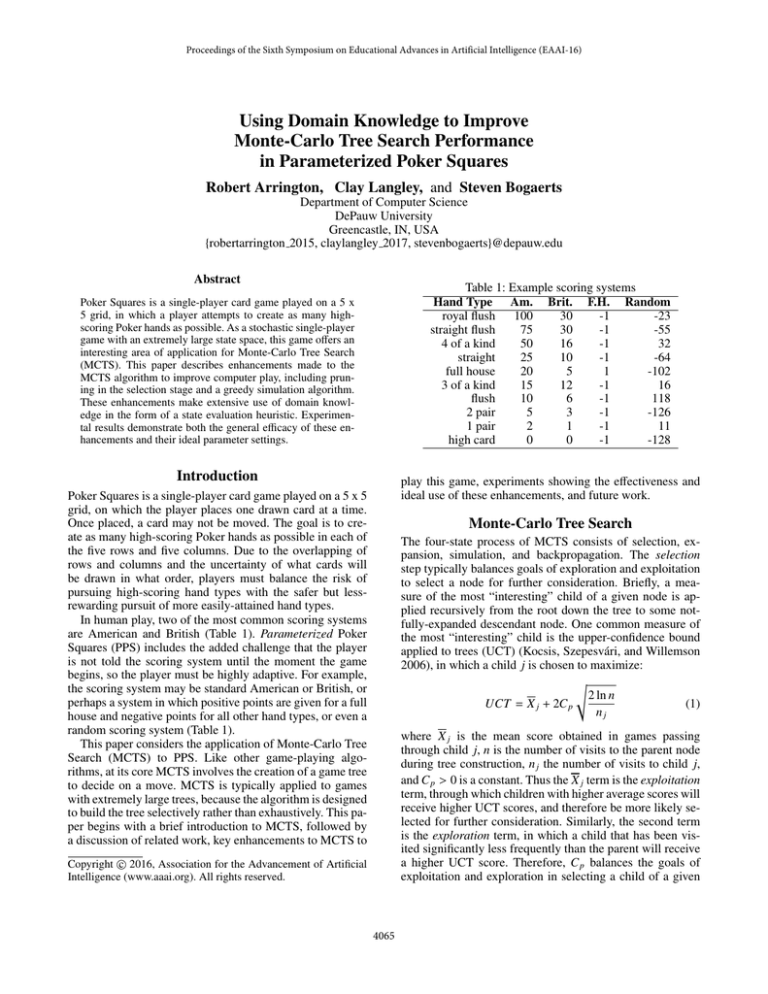
Table 1: Example scoring systems
Hand Type Am. Brit. F.H. Random
royal flush
100
30
-1
-23
straight flush
75
30
-1
-55
4 of a kind
50
16
-1
32
straight
25
10
-1
-64
full house
20
5
1
-102
3 of a kind
15
12
-1
16
flush
10
6
-1
118
2 pair
5
3
-1
-126
1 pair
2
1
-1
11
high card
0
0
-1
-128
Poker Squares is a single-player card game played on a 5 x
5 grid, in which a player attempts to create as many highscoring Poker hands as possible. As a stochastic single-player
game with an extremely large state space, this game offers an
interesting area of application for Monte-Carlo Tree Search
(MCTS). This paper describes enhancements made to the
MCTS algorithm to improve computer play, including pruning in the selection stage and a greedy simulation algorithm.
These enhancements make extensive use of domain knowledge in the form of a state evaluation heuristic. Experimental results demonstrate both the general efficacy of these enhancements and their ideal parameter settings.
Introduction
play this game, experiments showing the effectiveness and
ideal use of these enhancements, and future work.
Poker Squares is a single-player card game played on a 5 x 5
grid, on which the player places one drawn card at a time.
Once placed, a card may not be moved. The goal is to create as many high-scoring Poker hands as possible in each of
the five rows and five columns. Due to the overlapping of
rows and columns and the uncertainty of what cards will
be drawn in what order, players must balance the risk of
pursuing high-scoring hand types with the safer but lessrewarding pursuit of more easily-attained hand types.
In human play, two of the most common scoring systems
are American and British (Table 1). Parameterized Poker
Squares (PPS) includes the added challenge that the player
is not told the scoring system until the moment the game
begins, so the player must be highly adaptive. For example,
the scoring system may be standard American or British, or
perhaps a system in which positive points are given for a full
house and negative points for all other hand types, or even a
random scoring system (Table 1).
This paper considers the application of Monte-Carlo Tree
Search (MCTS) to PPS. Like other game-playing algorithms, at its core MCTS involves the creation of a game tree
to decide on a move. MCTS is typically applied to games
with extremely large trees, because the algorithm is designed
to build the tree selectively rather than exhaustively. This paper begins with a brief introduction to MCTS, followed by
a discussion of related work, key enhancements to MCTS to
Monte-Carlo Tree Search
The four-state process of MCTS consists of selection, expansion, simulation, and backpropagation. The selection
step typically balances goals of exploration and exploitation
to select a node for further consideration. Briefly, a measure of the most “interesting” child of a given node is applied recursively from the root down the tree to some notfully-expanded descendant node. One common measure of
the most “interesting” child is the upper-confidence bound
applied to trees (UCT) (Kocsis, Szepesvári, and Willemson
2006), in which a child j is chosen to maximize:
2 ln n
(1)
UCT = X j + 2C p
nj
where X j is the mean score obtained in games passing
through child j, n is the number of visits to the parent node
during tree construction, n j the number of visits to child j,
and C p > 0 is a constant. Thus the X j term is the exploitation
term, through which children with higher average scores will
receive higher UCT scores, and therefore be more likely selected for further consideration. Similarly, the second term
is the exploration term, in which a child that has been visited significantly less frequently than the parent will receive
a higher UCT score. Therefore, C p balances the goals of
exploitation and exploration in selecting a child of a given
c 2016, Association for the Advancement of Artificial
Copyright Intelligence (www.aaai.org). All rights reserved.
4065
node. Again, UCT can be applied recursively starting at the
root to traverse to a not-fully-expanded node in the existing
tree, thus completing the selection stage.
In expansion, a previously unconsidered child v of the selected node is randomly selected. In simulation, a game is
played from v to completion; in standard MCTS, simulation
consists entirely of random moves. Finally, in backpropagation, results of the simulation are used to update all nodes
on the path from v up to the root: each node’s visit count n
is incremented and average score Q is updated based on the
result of the simulated game. In this way, the tree is gradually and selectively developed, providing an increasingly
detailed picture of the expected score from various states in
the state space. Upon reaching some limit condition, a child
of the root can be selected based on any of a number of criteria, such as highest Q or highest n. For a detailed discussion
of the MCTS algorithm, see (Browne et al. 2012).
game to 30 seconds in total, both to make significant experimentation more manageable, and to maintain eligibility for
an upcoming PPS computer player contest.
For the first, second, next-to-last, and last moves, some
simple rules are used rather than the full MCTS process. For
the remaining moves, our “core” implementation of MCTS
uses no domain knowledge in selection nor simulation. We
describe next some enhancements on this core application
of MCTS, in which domain knowledge is added to both selection and simulation. This is followed by a discussion of
experimental results for these enhancements.
Domain Knowledge
While one benefit of the core MCTS algorithm is that very
little domain knowledge is required, nevertheless great performance improvements can be obtained with additional
knowledge. This subsection describes a PPS state-evaluation
heuristic, with the following subsections describing its application to simulation and selection.
A state is evaluated by adding the scores of each of its
ten Poker hands. Thus a state-evaluation heuristic is the sum
of ten applications of a hand-evaluation heuristic. When the
hand in question contains five cards, the system must simply
determine what hand type is represented, and look up the
corresponding score for the current scoring system.
For hands containing one to four cards, we first calculate a possibility array. This array contains one slot for each
hand type, from high card to royal flush. In each slot, 0 indicates that the hand type is no longer possible, 1 indicates
the hand type is possible, and 2 indicates the hand type is already made. For example, if a hand contains one card only,
then high-card is 2 and all other elements are 1, except that
royal flush may be 0 if the card is lower than ten and not an
ace. If a second card placed in the hand produces a pair, then
high-card and any hand types involving a straight would become 0, while pair would become 2. In turn, as more cards
are added, additional hand types may become impossible.
Four-card hands use the possibility array in a different
way than do one-, two-, and three-card hands. For each of
the hand types, a weight in [0, 1] is calculated, representing a rough measure of the likelihood of obtaining that hand
type with the next card draw. For a hand type with a 0 in
the possibility array, the weight is set to 0. For a hand type
with a 1 in the possibility array, the cards remaining in the
deck are analyzed to determine the weight. For example, if
a hand needs a 10 or 10♣ to complete a full house, and the
remaining cards in the deck include a 10 and five different
♠ cards, then the weight for a full house is calculated as 1/6.
For a hand type with a 2 in the possibility array (a hand
type that has already been achieved), the weight is not necessarily set to 1. For example, suppose a 4-card hand contains
a 6, 6♣, 6♠, and 7♠, while the deck contains only a 6, 7,
and 8. Here, the weight of three-of-a-kind, four-of-kind,
and full house would all be 1/3, since one of the three remaining cards in the deck leads to each of these hand types.
Once these weights are calculated for every hand type,
each weight is multiplied by the hand type value according
to the current scoring system, and added together to form a
weighted sum. Note that these calculations ignore the fact
Related Work In MCTS
Much prior work in MCTS has applied pruning to the game
tree. In soft pruning, a suboptimal node is hidden from consideration, but can be brought back if warranted by later reevaluation. In contrast, hard pruning offers no possibility for
bringing a pruned node back (Browne et al. 2012). Most
commonly, the node’s Q value is used in making pruning
decisions, but (Huang et al. 2010) describe alternative soft
(“relative”) and hard (“absolute”) pruning techniques based
on the visit count n.
Additional pruning strategies using domain knowledge
have been applied to the multi-player card game Lords of
War (Sephton et al. 2014). In this work, state evaluations
based on card counting are used to prune states that are less
likely to be useful. This work also considers the additional
time required for such evaluations – time that could be spent
further exploring the tree. Significant improvements are obtained with pruning despite this trade-off.
Simulation strategies enhanced with domain knowledge
have also been useful in MCTS research. For example, in
(Winands, Bjornsson, and Saito 2010) an MCTS player for
the strategy game Lines of Action uses a simulation that was
cut short, backpropagating a heuristic evaluation prior to the
end of the game rather than playing to completion. Another
approach is to use a heuristic to guide simulation, rather
than choosing moves randomly. For example, (Schadd et al.
2012) reports a 50% increase in average score in the game
SameGame when an accurate heuristic was added.
MCTS Application to PPS
Our MCTS application to PPS is built on top of the code
in (Hughart 2012), used under the MIT software license. The
MCTS algorithm is run each time a move is needed. The
tree begins with a choice node at its root, in which the current card must be placed in the grid. The children are chance
nodes, representing the random drawing of the next card to
be played, with alternating choice and chance nodes through
the remaining levels of the tree. This tree is gradually and selectively developed by repeatedly executing the four stages
of MCTS, with UCT in the selection stage. We limit each
4066
that the ten hands in the grid are dependent on each other.
This dependence is due to overlap of the rows and columns
on the grid, and occasional “competition” between hands for
the same card. Nevertheless, this calculation gives a reasonable heuristic for the evaluation of four-card hands.
This approach gets much more computationally intensive
for hands with fewer than four cards, and so in this case we
instead use estimated a-priori probabilities of hand types as
weights. We estimated these a-priori probabilities from the
British scoring system for Poker Squares, which is based
on the difficulty of finishing each of the hand types. (Note
that Poker Squares probabilities are not the same as Poker
probabilities.) These probabilities are then used to compute
a weighted sum in the same way as in a four-card hand.
These calculations can readily accommodate any scoring
system as a parameter. For example, if three-of-a-kind is valued at -100 points, then a high weight for three-of-a-kind
would lead to a significant drop in the weighted sum. Thus
this heuristic is highly adaptive to any scoring system.
Note, however, that there should be some value distinction between one-, two-, and three-card hands. For example,
a one-card hand will have nearly all, if not all, hand types
listed as “possible” in the possibility array. A two-card hand
will likely list fewer hand types as possible, and a three-card
hand fewer still. Yet a three-card hand is closer to completing its possible hand types than is a two- or one-card hand,
even with the same values in the possibility array. So all
else being equal, a three-card hand should be weighted more
highly. To account for this, we apply weights α, β, and γ
for one-, two-, and three-card hands, respectively. While we
would expect that 0 < α < β < γ < 1, ideal values are
the subject of experiments described later. In an initial implementation, we fix these values at α = 0.2, β = 0.4, and
γ = 0.6.
In practice, this sometimes leads to over-pruning. For example, if a drawn card does not fit well in any open space,
all children may have lower heuristic scores than the parent.
Thus an additional safeguard is used, that no more than 70%
of the children of any given parent may be pruned. If the
δ · h(p) threshold prunes more than this amount, then only
the bottom 50% of the children are pruned.
Modified Simulation
While the core MCTS implementation uses a completely
random game in the simulation step, the state heuristic can
also be applied to alternative simulation strategies. A pruning simulation strategy can apply the same pruning described above to simulation, such that a move is randomly
chosen from among the non-pruned children. Alternatively,
a best move simulation can be applied, in which all children are evaluated with the state heuristic, and the highestscoring child is taken as the choice in simulation. The tradeoff of these approaches, of course, is that they are more
computationally-intensive, and thus fewer iterations of the
MCTS process can be completed in a given time period.
Experiments and Analysis
The modifications to the core MCTS algorithm described
in the previous section are evaluated experimentally here.
We begin with a discussion of the exploration-exploitation
trade-off, followed by the use of domain knowledge in both
simulation and selection.
The Exploration–Exploitation Tradeoff
Recall from equation (1) that MCTS with UCT attempts to
balance the exploitation of relatively effective paths with the
exploration of lesser-known paths. This balance is controlled
via the constant C p , where a higher value means a stronger
emphasis on exploration. As discussed previously, (Kocsis,
√
Szepesvári, and Willemson 2006) suggest that C p = 1/ 2
is ideal when rewards range in [0, 1].
In some games, a reward range in [0, 1] is straightforward.
For example, 0 could mean a loss, and 1 a win, or maximum
and minimum possible scores could be translated to 0 and 1,
respectively, to “squash” the scores.
Unfortunately in PPS, squashing to the [0, 1] range is not
straightforward. To find the maximum score, for example, a
first attempt might be to simply take ten times the maximumscoring hand. For example, with the American scoring system (Table 1), this would be 1,000. Of course it is not possible to have ten royal flushes in a 5 × 5 grid, due to the dependence between hands and the use of a single deck of cards.
In fact, in the American scoring system, the maximum score
is 725, corresponding to four royal flushes, a straight flush,
and five four-of-a-kinds. In a more unusual scoring system,
a different set of hands might be higher-scoring. So finding
a maximum (or minimum) for squashing is not trivial.
Compounding this problem is the difference between the
maximum possible score and the most likely scores. In some
scoring systems, scores close to the maximum may be easy
to achieve – for example, in a scoring system in which only
Modified Selection Through Pruning
Recall in our core MCTS implementation that the selection
process uses UCT to find a not-fully-expanded node. This
means that nodes with low visit counts are favored, to some
extent even when observed rewards are low. While some
other games do have significantly higher branching factors
than PPS, there is still potentially much to gain through
pruning. The state heuristic can be used for this purpose.
As discussed previously, there are two typical strategies
for pruning: soft pruning, in which pruned nodes may be
brought back, and hard pruning, in which pruned nodes are
lost forever. While soft pruning may have some benefits, the
decision of whether or not to bring a node back leads to extra
computation and knowledge requirements, and so we opt for
hard pruning in this work.
First we calculate the heuristic score h(p) for the parent.
The value δ · h(p), for some constant δ, is set as the heuristic score threshold for each child. All children below this
threshold are pruned, never to be considered for selection.
For example, δ = 0.9 would prune children with < 90% of
the score of the parent, while any δ > 1 would prune all children that do not improve over the score of the parent. For the
purposes of future experiments, we fix δ at 1.3.
4067
Table 2: Effect of Score Squashing
Method Range
Score
Precise 0 – 725
91
Imprecise 0 – 1000
91
Max 200 0 – 200
90
Max 2000 0 – 2000
90
high-card is worth positive points. In others, however, typical scores may be far lower than the maximum. In the American scoring system, for example, while 725 is the maximum possible, scores in the 100’s are much more common.
Squashing to the [0, 1] range would mean that a score of
100 would become 0.138, while a score of 150 would become 0.207. So most scores would be in a tight range, leaving the rest of the range up to 1 rarely used. This may have
unintended consequences in the UCT calculation, as nodes
would look more similar than they should due to this squashing under an unrealistically high maximum possible score.
Nevertheless, we did create multiple squashing algorithms to compare performance of various C p values with
and without squashing. Precise squashing calculates a precise minimum and maximum score in order to squash exactly to the [0, 1] range. Since this method is not trivial
across scoring systems, a faster yet less accurate imprecise
squashing method was also developed, in which the lowest
possible hand score was multiplied by 10 for the minimum,
and the highest hand score multiplied by 10 for the maximum. In testing the American scoring system, we also examined a simple hard-coded maximum of 200, and as a test
in absurdity, another squashing method using a maximum of
2,000 (2.76 times higher than the actual maximum of 725).
Each of these squashing mechanisms was tested with core
MCTS by playing 700 games
√ using the American scoring
system. C p was set to 1/ 2 as recommended for scores
in the [0, 1] range. Results are shown in Table 2. The table demonstrates minimal impact of squashing accuracy;
even the absurd maximum of 2,000 achieved fairly comparable results. This suggests that a simple imprecise squashing
method is sufficient.
This begs the question,
however, of whether squashing
√
and using C p = 1/ 2 is worthwhile at all. To explore this,
we tested various C p values without squashing on the American scoring system. As shown in Figure 1, the lowest C p
values have the worst results. For the American scoring system, at around 7.5, scores level off for the most part, with a
slight peak score of 95 around C p = 20. Pushing C p values
even higher leads to only a slight reduction in score; even
C p = 5000 (not shown in the figure) earned a mean score of
91 in the American scoring system. This can be explained by
noting that for any sufficiently high C p value, the exploration
term of equation 1 will dominate the exploitation term, and
so further increases in C p have little effect.
It is also interesting to note that the best scores in Figure 1
are a bit higher than the scores in Table 2. This is likely due
to the issues described previously, that in games that do not
use the full range of scores, squashing can be problematic.
While the squashing procedure could likely be tuned pre-
Figure 1: Mean score (American system) for various C p
cisely to achieve a higher score, it seems simpler in this case
to achieve the same by adjusting the single variable C p .
The goal of these experiments was to fix a C p value for
the experiments that follow. Figure 1 suggests that around
C p = 20 is the best value for American scoring. Since other
scoring systems will have different typical scores, the ideal
setting will vary by system. Figure 1 does suggest, however,
that reasonably good performance can be achieved for any
C p value above some minimum dependent on the scoring
system. Since we are designing a player to be effective
under
√
any system, we choose a fairly high C p = 200/ 2 = 141.4
and focus on other parameters in the remainder of this paper,
rather than creating a more dynamic C p at this time.1
Computational Cost of the Heuristic
As described above, the state-evaluation heuristic can be applied to create alternative selection and simulation strategies.
Of course, heuristic calculations come at a computational
cost, with more time required per iteration of the MCTS process, and therefore fewer iterations total in a given amount
of time. So we start by examining the practical cost of the
heuristic calculation itself.
We do this by considering heuristic calculations but not
applications to any enhanced selection or simulation strategy. Table 3 shows results for the American scoring system,
with rows (1) – (4) addressing the issue of heuristic calculation cost. Row (1) reflects standard MCTS, with UCT-based
selection and random simulation. Rows (2) – (4) also use
these standard strategies, but with the “+ Calc.” notation indicating that the heuristic calculations are performed but not
actually applied to any pruning or simulation enhancements.
The drop in scores in rows (2) – (4) compared to row (1)
gives a reasonable indication of the cost of spending time on
heuristic calculations rather than more iterations of MCTS.
This deficit is 13 points (comparing rows (1) and (4)) in the
American scoring system when the heuristic is calculated in
1
This value was originally chosen based on the idea that 200 is
often considered a “winning” score in the American system, and
thus we were comparing it to a squashed value of 1. In practice this
value gave good results across scoring systems, and so its use was
continued, although other values would be appropriate as well.
4068
Table 3: Selection and simulation results over 2,000 games
Row
(1)
(2)
(3)
(4)
(5)
(6)
(7)
(8)
(9)
(10)
(11)
(12)
Selection
UCT
UCT + Calc.
UCT
UCT + Calc.
UCT
UCT
Best Move
Prune + UCT
Prune + UCT
Prune + UCT
UCT
Prune + UCT
Simulation
Random
Random
Random + Calc.
Random + Calc.
Prune + Random
Best Move
Random
Random
Best Move
Random
Best Move
Best Move
Mean Score
92
90
80
79
95
112
72
91
113
94*
118*
123*
both selection and simulation.
The data also show that the cost of adding calculations
to selection is around just 1 or 2 points – the difference
between rows (3) and (4), and between rows (1) and (2),
respectively. The cost of adding calculations to simulation,
however, is much higher, at around 11 or 12 points – the difference between rows (2) and (4), and between rows (1) and
(3), respectively. This makes sense, as for each time that selection does the calculations, the simulation will do them
several times – once for every move in the remainder of
the game. Thus any enhancement to selection or simulation
must overcome the deficit of the added calculation cost before being worthwhile, with simulation enhancements having a much greater deficit to overcome than selection enhancements. The following subsections explore the extent
to which some enhancements overcome this deficit.
Figure 2: α, β, and γ for each resulting mean score.
is capable of suggesting. In contrast, prune + random gives
the heuristic less control, only determining a set of higherscoring moves from which a random selection is made.
Domain Knowledge and Selection
This next set of experiments considers the application of the
state heuristic to the selection step of MCTS. We consider
best move selection, in which only the best child (according to the heuristic) is available for selection. We also consider prune + UCT selection, in which the heuristic is used
to prune children below a threshold as described previously.
Consider again Table 3. Row (7) shows that with a score
of 72, best move selection is highly ineffective, scoring even
worse than row (2) in which the calculations are performed
but not applied. This is not surprising, since such a drastic
approach severely limits the number of nodes available for
exploration. While best move simulation is a useful limitation in contrast to random simulation, the more principled
exploration of selection with UCT should not be so severely
restricted by a best move approach.
With a mean score of 91 (row (8)), prune + UCT selection shows little improvement over the non-application of
the calculations (90 in row (2)) and a slight loss compared
to standard MCTS (92 in row (1)). However, it is also interesting to consider rows (6) and (9). Using best move simulation instead of random simulation, there is a 1 point increase,
rather than decrease, in using prune + UCT selection. Taken
together, these results lead us to conclude that the application of prune + UCT as defined here is a wash – the benefit is
approximately equivalent to the cost. We will return to this
issue and show slight improvement with a more tuned prune
+ UCT in the final set of experiments.
Domain Knowledge and Simulation
The state-evaluation heuristic can be used to create alternatives to random simulation. One such alternative, prune +
random simulation, randomly selects each move not from
the complete set of possible moves, but rather from a smaller
set of nodes after pruning those scored beneath a threshold.
The pruning technique used is the same as that previously
described for selection. Another option is best move simulation, in which the highest-scoring move is always chosen.
Rows (1), (3), (5), and (6) of Table 3 show the relevant
results for these simulation experiments. Note prune + random simulation’s mean score of 95 (row (5)) shows some
improvement over the 92 of standard MCTS (row (1)). This
is more striking when considering that prune + random’s 95
actually overcame the drop down to 80 of the added heuristic
calculation cost (row (3)).
Even more impressive, however, are the gains for best
move simulation (row (6)). This approach earned a mean
score of 112, significantly higher than the calculation deficit
score of 80 (row (3)) and the standard MCTS score of 92
(row (1)). This demonstrates that, despite the added cost of
the heuristic calculations, they are quite worthwhile in a best
move simulation strategy.
It seems intuitive that best move simulation is more effective than prune + random, since best move plays a simulated game according to the best choices that the heuristic
Further Tuning of Domain Knowledge
This set of experiments considers further tuning of the
heuristic while using prune + UCT selection and best move
simulation. Recall that thus far heuristic parameters are fixed
4069
be improved and are worthwhile after tuning to the domain.
Conclusion and Future Work
This paper has described the application of MCTS to Parameterized Poker Squares. Experiments show that with
carefully-tuned domain knowledge, pruning in selection and
a best move simulation lead to significant improvements in
performance. These improvements overcome the added cost
of these strategies, particularly in simulation.
This work generates a number of interesting follow-up
questions for further research. Further experiments on the
pruning threshold policy (including the δ value) may tune
the pruning procedure for even more gains. The heuristic
could also be explored further in comparing 3-card and 4card hand evaluations. The experiments on C p values warrant further exploration and perhaps generalization to other
games in the hope of identifying best practices when squashing to [0, 1] is challenging. Experiments on other scoring
systems suggest the results of this paper are very applicable in general, but minor variations exist that could be exploited in further tuning. Finally, given the significant timeconstraints of the PPS player described here, significant
gains may be found in applications of parallelism.
Figure 3: β : α and γ : β for each resulting mean score.
at α = 0.2, β = 0.4, and γ = 0.6 for the weighting
given to one-, two-, and three-card hands, respectively. For
brevity, we denote this here as [0.2, 0.4, 0.6]. This section
considers various settings of these parameters. We constrain
α ≤ β ≤ γ, and consider both parameter magnitudes and the
ratios β : α and γ : β in selecting experimental settings.
Figures 2 and 3 show results of these experiments for the
American scoring system. For example, with [0.05, 0.4, 0.6],
a mean score of 109 was obtained. This corresponds to the
three left-most data points in Figure 2, where vertical placement of the symbols indicates parameter settings, and horizontal placement indicates mean score. In Figure 3, since
β : α = 8.0 and γ : β = 1.5 for [0.05, 0.4, 0.6], the two
leftmost ratio symbols are at vertical points 8.0 and 1.5.
Note in both figures that the results are fairly scattered
on the left side where mean scores are lower, yet somewhat more uniform on the right side where mean scores are
higher. This demonstrates a preference for certain parameter settings to obtain the highest scores. For example, in
Figure 2, nearly all higher-scoring players tend to converge
towards the highest-scoring player’s [0.1, 0.3, 0.85], with
stronger convergence in the α and β values. Some trends are
also visible in Figure 3, where the highest-scoring players
tend to have both weight ratios around 3. The highest scoring player attains a mean score of 123 in the American scoring system (row (12) of Table 3). The * next to the score in
the table indicates [0.1, 0.3, 0.85] rather than [0.2, 0.4, 0.6].
This is a strong improvement over the 113 of row (9).
We now return to prune + UCT selection, which seemed
ineffective in the results of the previous section. Row (10)
shows that prune + UCT selection with [0.1, 0.3, 0.85] attains a 94. This is compared to the 91 (row (8)) with
[0.2, 0.4, 0.6], and the 92 (row (1)) of standard MCTS. Similarly, best move simulation with [0.1, 0.3, 0.85] scores 118
(row (11)), showing further improvement over the 112 (row
(6)) with [0.2, 0.4, 0.6]. These experiments demonstrate that
both prune + UCT selection and best move simulation can
References
Browne, C. B.; Powley, E.; Whitehouse, D.; Lucas, S. M.;
Cowling, P.; Rohlfshagen, P.; Tavener, S.; Perez, D.;
Samothrakis, S.; Colton, S.; et al. 2012. A survey of monte
carlo tree search methods. Computational Intelligence and
AI in Games, IEEE Transactions on 4(1):1–43.
Huang, J.; Liu, Z.; Lu, B.; and Xiao, F. 2010. Pruning in
uct algorithm. In Technologies and Applications of Artificial
Intelligence (TAAI), 2010 International Conference on, 177–
181. IEEE.
Hughart, K. 2012. Uct for games. https://code.google.com
/p/uct-for-games/. Accessed: 2015-06-05.
Kocsis, L.; Szepesvári, C.; and Willemson, J. 2006. Improved monte-carlo search. Univ. Tartu, Estonia, Tech. Rep
1.
Schadd, M. P.; Winands, M. H.; Tak, M. J.; and Uiterwijk,
J. W. 2012. Single-player monte-carlo tree search for
samegame. Knowledge-Based Systems 34:3–11.
Sephton, N.; Cowling, P.; Powley, E.; and Slaven, N. 2014.
Heuristic move pruning in monte carlo tree search for the
strategic card game lords of war. In Computational Intelligence and Games (CIG), 2014 IEEE Conference on, 1–7.
Winands, M. H.; Bjornsson, Y.; and Saito, J.-T. 2010. Monte
carlo tree search in lines of action. Computational Intelligence and AI in Games, IEEE Transactions on 2(4):239–
250.
4070