Proceedings of the Twenty-Seventh AAAI Conference on Artificial Intelligence
Compact RGBD Surface Models Based on Sparse Coding
Michael Ruhnke
Liefeng Bo
Dieter Fox
Wolfram Burgard
University of Freiburg
ruhnke@cs.uni-freiburg.de
ISTC-PC Intel Labs
liefeng.bo@intel.com
University of Washington
fox@cs.washington.edu
University of Freiburg
burgard@cs.uni-freiburg.de
Abstract
In this paper, we describe a novel approach to construct compact colored 3D environment models representing local surface attributes via sparse coding. Our method decomposes a
set of colored point clouds into local surface patches and encodes them based on an overcomplete dictionary. Instead of
storing the entire point cloud, we store a dictionary, surface
patch positions, and a sparse code description of the depth
and RGB attributes for every patch. The dictionary is learned
in an unsupervised way from surface patches sampled from
indoor maps. We show that better dictionaries can be learned
by extending the K-SVD method with a binary weighting
scheme that ignores undefined surface cells. Through experimental evaluation on real world laser and RGBD datasets
we demonstrate that our method produces compact and accurate models. Furthermore, we clearly outperform an existing
state of the art method in terms of compactness, accuracy,
and computation time. Additionally, we demonstrate that our
sparse code descriptions can be utilized for other important
tasks such as object detection.
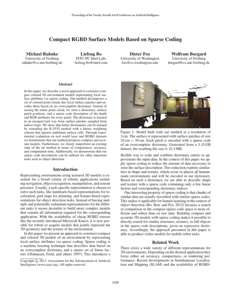
Figure 1: Model built with our method at a resolution of
2 cm. The surface is represented with surface patches of size
20 cm × 20 cm. Each patch is encoded with a sparse code
of an overcomplete dictionary. Generated from a 3.35 GB
dataset, the resulting file size is 10.2 MB.
flexible way to scale and combine dictionary entries to approximate the input data. In the context of this paper we apply sparse coding to reduce the amount of data necessary to
store the surface description. This reduction exploits similarities in shape and texture, which occur in almost all humanmade environments and will be encoded in our dictionary.
Based on such a dictionary we are able to describe shape
and texture with a sparse code containing only a few linear
factors and corresponding dictionary indices.
One interesting property of sparse coding is that chunks of
similar data are usually described with similar sparse codes.
This makes it applicable for feature learning in the context of
object detection (Bo, Ren, and Fox 2012) because a search
or comparison in the compact sparse code space is more efficient and robust than on raw data. Building compact and
accurate 3D models with sparse coding makes it possible to
directly search for similar structures, textures, or full objects
in the sparse code descriptions, given an expressive dictionary. Accordingly, the approach presented in this paper is
able to produce richer models for mobile robot tasks.
Introduction
Representing environments using textured 3D models is essential for a broad variety of robotic applications including navigation, object recognition, manipulation, and remote
presence. Usually, a task-specific representation is chosen to
solve such tasks, like landmark-based representations for localization, grid maps for planning, and feature-based representations for object detection tasks. Instead of having multiple and potentially redundant representations for the different tasks it seems desirable to build more complex models
that contain all information required for the corresponding
application. With the availability of cheap RGBD sensors
like the recently introduced Microsoft Kinect, it is now possible for robots to acquire models that jointly represent the
3D geometry and the texture of the environment.
In this paper we present an approach to construct compact
and colored 3D models of an environment by representing
local surface attributes via sparse coding. Sparse coding is
a machine learning technique that describes data based on
an overcomplete dictionary and a sparse set of linear factors (Olshausen, Field, and others 1997). This introduces a
Related Work
There exists a wide variety of different representations for
3D environments. Depending on the desired application they
focus either on accuracy, compactness, or rendering performance. Recent developments in Simultaneous Localization and Mapping (SLAM) and the availability of RGBD-
c 2013, Association for the Advancement of Artificial
Copyright Intelligence (www.aaai.org). All rights reserved.
1429
cameras made it possible to obtain large colored metric models. Whereas a major advantage of colored point-clouds lies
in their accuracy, their drawback is the amount of data that
has to be stored, since every single observed pixel is represented in both 3D and RGB-space. Therefore, most RGBDbased SLAM systems either use only a subset of features
internally (Henry et al. 2010) or represent only small, local
spaces (Newcombe et al. 2011).
Fairfield, Kantor, and Wettergreen (2007) proposed a
compact voxel representation based on Octrees in the context of mobile robotics. Wurm et al. (2010) developed an
open source implementation called Octomap which can
store additional RGB information together with 3D occupancy. Kammerl et al. (2012) used Octrees to compress colored point cloud streams by transmitting only the differences
in successive frames. For large voxel sizes, Octrees are very
compact but introduce major discretization errors. If a small
voxel size is chosen the resulting models are more accurate
but not compact anymore.
In our previous work Ruhnke et al. (2010) we proposed
to model the geometric structure of an environment based
on surface primitives. In this approach, a surface primitive is
a small point cloud that can be inserted in a model at multiple locations. The corresponding model uses a dictionary
of primitives and stores a set of 6 degrees of freedom locations together with the corresponding dictionary indices,
describing where to place which of the small point clouds to
reconstruct the input data. In principle, this can be regarded
as a variant of bag-of-words models.
A technique similar to bag-of-words methods is sparse
coding. Instead of choosing one dictionary entry of a bagof-words to describe an input signal, sparse coding allows
to describe a signal as a linear combination of multiple dictionary entries. Sparse coding has already been successfully
applied in the context of signal approximation (Rubinstein,
Zibulevsky, and Elad 2010), image denoising (Hyvarinen,
Hoyer, and Oja 2001; Elad and Aharon 2006) and more recently to learn feature descriptions for object recognition
tasks on both vision only and RGB-D data (Bo, Ren, and
Fox 2012; Yang et al. 2009); resulting in superior recognition results compared to standard bag-of-words models.
In this work, we follow a similar idea to describe models as a set of local descriptions. However, in contrast to our
previous work Ruhnke et al. (2010), we use discrete local
surface descriptions and apply sparse coding to approximate
the surfaces. Instead of a greedy dictionary learning using
the Bayesian information criterion to guide the search, we
apply an efficient variant of K-SVD (Rubinstein, Zibulevsky,
and Elad 2008) and learn smaller dictionaries while achieving substantially lower reconstruction errors. In addition, our
method is also able to represent full RGB-D information instead of just the 3D surface model.
Figure 2: Example RGB-D patch (left), the depth description
(center) and the color description (right). The light green areas on the center and right image correspond to undefined
areas, which are marked as zeroes in the patch bitmask.
a dictionary from the surface patches as reference for our
codes. Once we have a dictionary, we approximate the surface patches with sparse codes referring to that dictionary.
Given the locations, the dictionary, and the sparse codes, we
can approximate every patch and place it at the right location
to recover the entire surface model of the environment.
In our context, the input data is a pre-registered set of colored point clouds P. To apply sparse coding, we first decompose P into chunks of a particular size and discretize
every chunk. Typical ways for doing this are by considering
pixel or metric space. Since we intend to jointly represent
the information from multiple point clouds acquired at different locations, choosing pixel space would result in differently scaled surface descriptions, making it hard to combine
the surface information observed from multiple scans. On
the other hand, a discretization in metric space has the disadvantage of introducing additional errors since we usually
observe nearby surfaces at very high resolutions and store
the information at a lower resolution.
We represent the surface with small RGB-D patches of a
given size and a fixed metric resolution on the surface. The
depth and RGB values are oriented in the direction of the
surface normal. In this way, we discretize only in the two
dimensions of the surface and have full accuracy in the third
dimension. Let us consider a surface patch of size 10 cm
×10 cm with a resolution of 1 cm. In our surface representation this would result in a 10 × 10 matrix for the depth
channel and a 10 × 10 × 3 matrix for the color channel. Figure 2 shows an example surface patch and the corresponding
depth and color channels.
To describe a set of colored point clouds, P, we define
a model M(Ddepth , Drgb , I) that contains reference dictionaries for both channels, Ddepth and Drgb , and a scene
of the
description I = {i1 , . . . , il }. The entries ddepth
i
depth
depth dictionary Ddepth = {ddepth
,
.
.
.
,
d
}
have
the
n
1
same size as the depth channels of the surface patches.
Likewise, the entries drgb
of the RGB dictionary Drgb =
i
rgb
{d1 , . . . , drgb
m } have the same size as the surface patch
color channel. Since shape has less variations than texture,
rgb
Ddepth has usually
substantially less entries than D .
Sparse Coded 3D Surface Models
Every ij = Tj , cdepth
stores a transforma, crgb
j
j , bj
tion, consisting of 3D pose and orientation, for the surface
patch, Tj , one sparse code for the depth cdepth
and one for
j
,
and
a
bitmask
b
that
is
1 for dethe RGB channel crgb
j
j
fined cells and 0 for undefined cells (see also Figure 2). Note
The main goal of our method is to build 3D surface models based on sparse coding. In the following we will refer to
local surfaces as surface patches, or simply patches. Such
patches need a well defined location in order to compute
them from the input data. Furthermore, we need to learn
1430
Algorithm 1 Pseudo code for patch location computation.
1: S = ∅
2: for all points p ∈ P do
3:
Insert p into voxel v ∈ V ;
4: compute centroids c ∈ C for all non-empty voxels;
5: for all centroids c ∈ C do
6:
for all neighboring centroids n ∈ C do
7:
if ||c − n||22 < minDistance then
8:
c := c+n
2 and remove n from C;
9:
if ||c − n||22 > maxDistance then
10:
add c+n
2 to set of locations;
11:
add c to set of patch locations S;
12: return S;
Figure 3: Colored point cloud and corresponding surface
patch locations. The blue axis corresponds to the normal.
that undefined cells can be caused by invalid range measurements of the sensor, occlusions, or if measurements are too
far away (background). In this way we can decouple the impact of occlusions from the surface description and get sharp
surface borders. The storage requirements are rather moderate. Given a patch size of 10 × 10 we have to store 100 bits
or 12 Byte, which corresponds to three floats per extracted
surface patch.
In the following we will discuss how we partition the input data, learn a dictionary from the extracted patches and
calculate a sparse description for every patch.
responding eigenvectors are not well defined and tend to be
strongly influenced by sensor noise. To avoid this situation,
we select alternative local x- and y-axes by choosing the
two global coordinate axes that have the larger angle to the
computed normal and make them orthogonal to the normal.
This results in more regular surface patch orientations on
flat surfaces. If less than three points fall into one patch location we set the rotation to the identity matrix. Combining
the patch location and the computed orientation, we can define a transformation Ti as a local coordinate frame of our
surface patch. A typical result of this procedure can be seen
in Figure 3. Once we computed Ti , we apply Ti−1 to the
point cloud neighborhood and compute the color and depth
value for each cell in the patch by averaging over the points
falling into that cell (empty cells are marked as undefined).
Point Cloud Decomposition
To decompose a point cloud P into a set of surface patches,
S, we have to decide where to place the surface patches si .
Each surface patch describes a subset of points of P that fit
into a cube of a particular size. Possible locations for the
surface patches are defined by the points in P. For compressing the data we are interested in the minimum number
of subsets that contain all elements of P and the locations of
those subsets. This is a set cover problem known to be NPcomplete (Feige 1998). Instead of searching for an optimal
solution we focus on a computationally efficient, approximate solution. Note that P may contain millions of points
and that the computation of surface patches for every point
is already expensive in terms of computation time and memory requirements. Therefore, we uniformly distribute the locations for our surface patches on P and keep the amount of
overlapping regions relatively low. We perform this using a
spatial sub-sampling strategy and a voxel grid as described
in Algorithm 1. The neighborhood of the centroids is defined
by the voxel grid, and steps 8 and 10 merge or add centroids
in case neighbors are too close or too far apart, respectively.
Dictionary Learning with wK-SVD
The extracted surface patches S contain a lot of redundant
information on both channels. Thus, we intend to compute a
sparse approximation to find a compact representation of the
data. Let S be the data matrix that contains every si as i-th
column vector. The idea of K-SVD is to learn an overcomplete dictionary D and a sparse description X to approximate S. We can formulate this as a minimization problem
using the following equation:
2
min S − (W (DX))F
s.t. ∀i xi 0 ≤ k.
(1)
Here, AF denotes the Frobenius norm, denotes the
element-wise matrix multiplication, and k is the maximum
number of nonzero entries for each column xi that approximates a corresponding surface patch si ≈ Dxi . To deal with
undefined values we extend the standard K-SVD formulation with a binary weighting matrix W that contains a 1 for
data cells that were actually observed and 0 otherwise. This
information is represented in the bitmasks of the patches.
In this way we ignore the reconstruction results for undefined values and focus the reconstruction accuracy on the
observed values. Undefined cells store a value of zero in S
and by multiplying W in an element-wise fashion we ensure
that the reconstructed values of undefined cells are ignored
during the optimization. In the following we will briefly outline weighted K-SVD (wK-SVD) and describe the proposed
extension. Pseudo code of wK-SVD is provided in Algorithm 2. A more detailed description of an efficient K-SVD
Once patch locations are determined, we calculate a surface patch si for every such location. Additionally, we need
to compute the orientation and rotation of the surface around
every patch location. Therefore, we extract a local point
cloud for every patch location with a diameter similar to
our surface patch size and compute the mean and the covariance of this local point cloud. We compute the rotation
via a singular value decomposition (SVD) on the covariance.
The eigenvector of the smallest eigenvalue corresponds to
the normal and is used as the z-axis direction of the surface
patch. The remaining two eigenvectors correspond to the xand y-axes, in order of their ascending eigenvalues. Furthermore, we check the ratio between the two larger eigenvalues. If the ratio is close to one, the orientations of the cor-
1431
Dataset
Scene IV-A
Scene IV-A
RGBD Corridor
RGBD Corridor
Object Detect.
method
Ruhnke 2010
our method
Octomap
our method
our method
dict. (D/RGB)
70 / 70 / -/100 / 500
120 / 114k∗
patch size
0.1 m
0.16 m
0.2 m
0.1 m
res.(m)
0.02
0.02
0.02
0.005
input
1.2 MB
1.2 MB
3.35 GB
3.35 GB
4.7 MB
result
431 kB
357 kB
44.5 MB
10.2 MB
559 MB
RMSE (D/RGB)
0.058 m / 0.016 m / 0.016 m / 25.1
0.017 m / 19.9
-
time
7 min
2.5 s
56 s
8 min
5s
Table 1: Experimental evaluation for each dataset and method. The dictionary size and RMSE errors are split into depth and
RGB. The timings are measured on a standard desktop CPU with 3 GHz. (∗ ) The RGB channel was not compressed.
Algorithm 2 Pseudo code for wK-SVD algorithm.
1: Initial D0 filled with randomly selected columns of S
2: for all Iterations do
3:
for all xi ∈ X do compute sparse code matrix X
2
4:
xi = argmin si − (wi (Dxi ))2
5:
for all dj ∈ D do
optimize dictionary D
6:
L := Indices of X columns i with dj,i = 0
(L)
7:
SVD(S (L) − W (L) (DX (L) − dj Xrow(j) ))
8:
dj = SVD.getU().normalize()
(L)
9:
Xrow(j) = SVD.getS() · SVD.getV()
Bo, Ren, and Fox 2012).
Once all values of a model M(Ddepth , Drgb , I) are determined, we can also reconstruct a point cloud from it, if
needed. This can be done by going through all elements of
I and decode the j-th element with
sˆj depth = Ddepth · cdepth
.
j
(3)
With cdepth
= [λ1j , . . . , λN
j ] this can be rewritten as
j
depth
+ . . . + λN
.
sˆj = λ1j · ddepth
j · dN
1
(4)
Remember that the sparse code cj is a sparse vector with
only k nonzero entries. The same scheme is applied for decoding the color channel. The joint information is projected
into a colored 3D point cloud for all values defined in bj . In
the final step, we apply Tj to put the patch point cloud at the
right location in the resulting point cloud.
implementation without weighting can be found in the work
of Rubinstein, Zibulevsky, and Elad (2008).
Starting from an initial dictionary D0 , wK-SVD iteratively achieves an improved representation of S. In each iteration, wK-SVD alternates between computing the sparse
code matrix X based on the current dictionary and optimizing each dictionary entry based on the current sparse code
matrix. We compute the sparse code matrix X with orthogonal matching pursuit (OMP) (Pati, Rezaiifar, and Krishnaprasad 1993). OMP is a greedy algorithm that decouples
the computation of X into N sub-problems, one for every
data item si . This makes it easy to parallelize OMP, which
results in a major speedup in our implementation. Given a
dictionary D, OMP iteratively solves the following minimization problem:
Experiments
In this section we evaluate our method on various datasets.
The interesting evaluation quantities for this work are
mainly the accuracy and compactness of the resulting model
and the time needed to compute the result. To evaluate accuracy we use the root mean squared error (RMSE) of the
dictionary learning method wK-SVD, which is calculated
on the discrete surface patches and their approximations according to Eq. (1). While this error provides insights into
how close we get to the optimal solution given our discretization, we are additionally interested in the point level
error for comparison with other methods and discretizations.
Therefore, we search for every point in the resulting point
cloud for the nearest neighbor in the reference point cloud
and vice versa. We compute the RMSE for all pairs. To
demonstrate how compact the results are, we provide the file
sizes of the input dataset and the resulting files in their corresponding representation in Table 1. Furthermore, we provide timings required for learning the dictionary since this
is usually the computationally most expensive step. All results were computed on a standard desktop machine with an
i7 CPU at 3 GHz and with four cores. In all experiments we
chose a sparsity factor of k = 5.
2
x̂i = argmin si − (wi (Dxi ))2 s.t. xi 0 ≤ k (2)
Again, we added a weighting vector wi , which is the i-th
column of the weighting matrix W used to neglect undefined values. In every iteration we search for the code word
that best matches the current residual and append it to the
current xi . Once a new code word is selected, the patch si
is orthogonally projected to the span of the selected code
words, and the residual is recomputed for the next iteration
until either the maximum number of entries k is reached or
the residual error is below a minimum error.
Once the sparse code matrix X is computed, wK-SVD updates the dictionary on a per-entry base. For each dictionary
entry dj , it only selects the patches that have a non-zero entry in their sparse code. A codeword dj is updated via SVD
on the residual matrix containing all differences between the
selected patches and their approximations using all codewords and their sparse codes without dj . In general, K-SVD
and wK-SVD can get stuck in a local minimum depending
on the initial dictionary. However, for practical scenarios,
K-SVD usually converges to a good dictionary for a wide
range of initializations (Aharon, Elad, and Bruckstein 2006;
Accuracy and Runtime vs. Dictionary Size
In our first experiment we evaluated the accuracy and runtime requirements of our method on a range only dataset. We
computed a point cloud decomposition containing 2,585 surface patches of size 16 cm and a resolution of 2 cm. To this
model we applied standard K-SVD and wK-SVD to learn a
dictionary. We varied the dictionary size between 1 and 901
1432
milimeter
15
10
5
0
0
180
160
140
120
100
80
60
40
20
0
10
10
depth RMSE in mm
RGB RMSE
9
milimeter
wK-SVD RMSE in mm
wK-SVD time
K-SVD RMSE in mm
K-SVD time
seconds
20
8
8
6
7
4
6
2
5
0
0
10
100 200 300 400 500 600 700 800 900
20
30
40
RGB values (0 - 255)
a)
b)
c)
Figure 4: The input point cloud of this experiment is shown in (a). The cloud contains only range information and the displayed
colors are height-dependent. The reconstruction quality of the method by Ruhnke et al. (2010) with a dictionary size of 70
is shown in (b). A model built by our method with a dictionary of the same size is shown in (c). As can be seen, the model
computed by our method maintains part of the original scan structure as a result of the stored bit masks and at the same time
provides a substantially better reconstruction accuracy. The resulting RMSE per point is approximately 1.6 cm and the resulting
file size is 357 kb compared to an RMSE of 5.8 cm and 421 kB achieved by Ruhnke et al. (2010).
50
iteration
Figure 6: RMSE of the depth and RGB dictionary learning
with wK-SVD. In both cases wK-SVD converges very fast
to an RMSE of 6 mm for depth and a RMSE of 4.5 for RGB.
dictionary size
Figure 5: Accuracy and time requirements for our method
on a range only reference dataset. We applied wK-SVD and
K-SVD with varying dictionary sizes between 1 and 901 and
a step size of 5. As can be seen, the RMSE of wK-SVD is
smaller than the RMSE of K-SVD for all dictionary sizes.
face patches instead of a sample point cloud for our dictionary entries. In this way, a depth value is stored with one
float instead of three in the point cloud representation. Furthermore, we use the gained space to store additional bitmasks and sparse codes with every surface description. Together this results in a better reconstruction quality.
with a step size of 5. Figure 5 gives a detailed overview of
the resulting RMSE per patch cell and the run time depending on the dictionary size. A dictionary of size 70 already
results in an RMSE of approximately 1 cm with a computation time around 2.5 seconds using four threads. The difference between wK-SVD and K-SVD is also very interesting.
The RMSE in the wK-SVD is smaller than for K-SVD for
all dictionary sizes, with a comparable run time.
Compact Models
In the next experimental setting we applied our method on
a SLAM solution1 containing 707 registered RGBD scans.
This dataset was acquired in the corridor of a typical office
building. An overview of the dataset can be seen in Figure 7(a). We applied our method to the accumulated point
cloud and built a model with 41,358 surface patches of size
20 cm and a resolution of 2 cm. It took eight minutes to compute the depth dictionary of size 100 and the RGB dictionary
of size 500. Figure 6 plots the evolution of the RMSE during
the dictionary learning for both dictionaries over the different iterations.
For comparison we created a colored occupancy Octomap
of the dataset with a voxel size of 2 cm, which resulted in the
colored model shown in Figure 7(c). An enlarged view of the
same region in our model is shown in 7(d). Our model looks
Figure 4(a) shows the input point cloud, (b) a model computed with the method described in (Ruhnke et al. 2010) and
(c) a model built by our method. Both methods used a dictionary of size 70. As can be seen, the model computed by
our method partially maintains the original scan structure
as a result of the stored bitmasks and additionally provides
a substantially better reconstruction accuracy. The resulting
RMSE per point is approximately 1.6 cm and the resulting
file size is 357 kb, compared to an RMSE of 5.8 cm and
a file size of 421 kb. Thus our method clearly outperforms
the competing approach in terms of the resulting file size,
the RMSE, and the time needed to learn the dictionary. The
main reason for the better results is that we use discrete sur-
1
1433
Courtesy of Peter Henry
a)
b)
c)
d)
Figure 7: Resulting model for the RGB Corridor dataset (a), a representative part of the model as a raw point cloud (b),
octomap (c) and our method (d). The Octomap occupancy grid has a file size of 44.49 MB with a voxel size of 2 cm, an RMSE
of 0.016 m on the depth channel and an RMSE of 25.1 on the RGB channel. Our model has a file size of 10.2 MB and stores a
depth dictionary with 100 entries and a RGB dictionary with 500 entries. The RMSE is 0.017 m for the depth channel and 19.9
for the RGB channel. In comparison, Octomap has a slightly lower error in the depth data and a slightly larger error in the RGB
data. The major difference between the two results is the resulting file size, which is four times larger for Octomap.
b)
c)
d)
a)
Figure 8: The RGBD scan used for this experiment is shown in (a). (b) shows the results for upper can parts search, (c) for
lower parts of a can standing on a flat surface and (d) shows the results for the edge of a table. The green cubes mark highly
similar surface patches for the corresponding search queries. In all three cases we successfully found all surface patches that
contain similar surface descriptions. Note that there is only one false positive in the lower part of the table leg shown in (d).
much smoother since we discretize only in two dimensions
and the sparse coding also reduces the noise in the RGB
data as can be seen on the wall on the left hand side. Furthermore, our model is substantially smaller with 10.2 MB
versus 44.5 MB.
the linear factor as similarity score. Furthermore, we show
only results with a value below a threshold of 0.05. As can
be seen for all three settings, our approach reliably found
similar surface patches. It produced only one false-positive
in the lower part of the table leg. This indicates that our approach can be applied for object recognition tasks despite the
simplistic nature of the detection algorithm. It furthermore
highlights the richer description of our models compared to
standard representations.
Object Detection
Since sparse coding has previously been applied successfully to object recognition, the question arises whether we
can also use our models to search for objects by comparing sparse codes. To evaluate this, we acquired an RGB-D
scan containing multiple small soda cans on a table (see
Figure 8(a)). To demonstrate similarities in the sparse code
space we extracted surface patches for every point in the
model instead of applying the proposed point cloud decomposition. In this way we avoid the problem of extracting the
sparse codes on suboptimal positions since our point cloud
decomposition scheme does not explicitly search for stable
key points or patch locations.
For a real object detection scenario one would compute
a model of the environment with our method along with a
reference model for the object we are searching for, with
surface patches in every point, based on the same dictionary.
In such a setting, we can find an object in an environment by
searching for surface patches that are very similar to a representative subset of the sparse description of the reference
model.
Figures 8(b), (c) and (d) show the results of three different search queries. The corresponding reference surface is
marked with a red cube, whereas the green cubes correspond
to the most similar surface patch regions. We forced an 80%
similarity on the indices and used the Euclidean metric on
Conclusions
In this paper, we presented a novel approach to construct
compact colored 3D environment models representing local
surface attributes via sparse coding. The key idea of our approach is to decompose a set of colored point clouds into
local surface patches and describe them based on an overcomplete dictionary. The dictionaries are learned in an unsupervised fashion from surface patches sampled from indoor maps. We demonstrate that our method produces highly
compact and highly accurate models on different real world
laser and RGBD datasets. Furthermore, we show that our
method outperforms an existing state-of-the-art method in
terms of compactness, accuracy and computation time. We
also demonstrate that our sparse code descriptions can be
utilized for other highly relevant tasks in the context of
robotics such as object detection.
Acknowledgments
This work was funded in part by the Intel Science and Technology Center for Pervasive Computing, by ONR MURI
grant N00014-07-1-0749 and by the EC under ERC-AGPE7-267686-LifeNav and FP7-ICT-248873-RADHAR.
1434
References
compact 3d map representation for robotic systems. In Proc.
of the ICRA 2010 workshop on best practice in 3D perception and modeling for mobile manipulation, volume 2.
Yang, J.; Yu, K.; Gong, Y.; and Huang, T. 2009. Linear spatial pyramid matching using sparse coding for image classification. In Computer Vision and Pattern Recognition, 2009.
CVPR 2009. IEEE Conference on, 1794–1801. IEEE.
Aharon, M.; Elad, M.; and Bruckstein, A. 2006. K-svd: An
algorithm for designing overcomplete dictionaries for sparse
representation. IEEE TRANSACTIONS ON SIGNAL PROCESSING 54(11):4311.
Bo, L.; Ren, X.; and Fox, D. 2012. Unsupervised feature
learning for RGB-D based object recognition. International
Symposium on Experimental Robotics (ISER), June.
Elad, M., and Aharon, M. 2006. Image denoising via sparse
and redundant representations over learned dictionaries. Image Processing, IEEE Transactions on 15(12):3736–3745.
Fairfield, N.; Kantor, G.; and Wettergreen, D. 2007. Realtime slam with octree evidence grids for exploration in underwater tunnels. Journal of Field Robotics 24(1-2):03–21.
Feige, U. 1998. A threshold of ln n for approximating set
cover. Journal of the ACM (JACM) 45(4):634–652.
Henry, P.; Krainin, M.; Herbst, E.; Ren, X.; and Fox, D.
2010. Rgb-d mapping: Using depth cameras for dense 3d
modeling of indoor environments. In the 12th International
Symposium on Experimental Robotics (ISER), volume 20,
22–25.
Hyvarinen, A.; Hoyer, P.; and Oja, E. 2001. Image denoising by sparse code shrinkage. Intelligent Signal Processing
554–568.
Kammerl, J.; Blodow, N.; Rusu, R. B.; Gedikli, S.; Beetz,
M.; and Steinbach, E. 2012. Real-time compression of
point cloud streams. In IEEE International Conference on
Robotics and Automation (ICRA).
Newcombe, R.; Davison, A.; Izadi, S.; Kohli, P.; Hilliges,
O.; Shotton, J.; Molyneaux, D.; Hodges, S.; Kim, D.; and
Fitzgibbon, A. 2011. Kinectfusion: Real-time dense surface
mapping and tracking. In Mixed and Augmented Reality (ISMAR), 2011 10th IEEE International Symposium on.
Olshausen, B.; Field, D.; et al. 1997. Sparse coding with an
overcomplete basis set: A strategy employed by vi? Vision
research 37(23):3311–3326.
Pati, Y.; Rezaiifar, R.; and Krishnaprasad, P. 1993. Orthogonal matching pursuit: Recursive function approximation with applications to wavelet decomposition. In Signals,
Systems and Computers, 1993. 1993 Conference Record of
The Twenty-Seventh Asilomar Conference on, 40–44. IEEE.
Rubinstein, R.; Zibulevsky, M.; and Elad, M. 2008. Efficient
implementation of the k-svd algorithm using batch orthogonal matching pursuit. CS Technion.
Rubinstein, R.; Zibulevsky, M.; and Elad, M. 2010. Double sparsity: Learning sparse dictionaries for sparse signal
approximation. Signal Processing, IEEE Transactions on
58(3):1553–1564.
Ruhnke, M.; Steder, B.; Grisetti, G.; and Burgard, W. 2010.
Unsupervised learning of compact 3d models based on the
detection of recurrent structures. In Proc. of the IEEE/RSJ
International Conference on Intelligent Robots and Systems
(IROS).
Wurm, K.; Hornung, A.; Bennewitz, M.; Stachniss, C.; and
Burgard, W. 2010. Octomap: A probabilistic, flexible, and
1435