Proceedings of the Twenty-Fourth AAAI Conference on Artificial Intelligence (AAAI-10)
Facial Age Estimation by Learning from Label Distributions
Xin Geng1,2,3 , Kate Smith-Miles1 , Zhi-Hua Zhou3∗
1
School of Mathematical Sciences, Monash University, VIC 3800, Australia
School of Computer Science and Engineering, Southeast University, Nanjing 210096, China
3
National Key Laboratory for Novel Software Technology, Nanjing University, Nanjing 210093, China
2
Abstract
One of the main difficulties in facial age estimation is
the lack of sufficient training data for many ages. Fortunately, the faces at close ages look similar since aging
is a slow and smooth process. Inspired by this observation, in this paper, instead of considering each face image as an example with one label (age), we regard each
face image as an example associated with a label distribution. The label distribution covers a number of class
labels, representing the degree that each label describes
the example. Through this way, in addition to the real
age, one face image can also contribute to the learning
of its adjacent ages. We propose an algorithm named
IIS-LLD for learning from the label distributions, which
is an iterative optimization process based on the maximum entropy model. Experimental results show the advantages of IIS-LLD over the traditional learning methods based on single-labeled data.
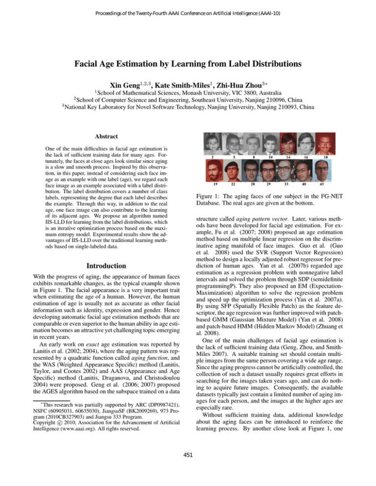
Figure 1: The aging faces of one subject in the FG-NET
Database. The real ages are given at the bottom.
structure called aging pattern vector. Later, various methods have been developed for facial age estimation. For example, Fu et al. (2007; 2008) proposed an age estimation
method based on multiple linear regression on the discriminative aging manifold of face images. Guo et al. (Guo
et al. 2008) used the SVR (Support Vector Regression)
method to design a locally adjusted robust regressor for prediction of human ages. Yan et al. (2007b) regarded age
estimation as a regression problem with nonnegative label
intervals and solved the problem through SDP (semidefinite
programmingP). They also proposed an EM (ExpectationMaximization) algorithm to solve the regression problem
and speed up the optimization process (Yan et al. 2007a).
By using SFP (Spatially Flexible Patch) as the feature descriptor, the age regression was further improved with patchbased GMM (Gaussian Mixture Model) (Yan et al. 2008)
and patch-based HMM (Hidden Markov Model) (Zhuang et
al. 2008).
One of the main challenges of facial age estimation is
the lack of sufficient training data (Geng, Zhou, and SmithMiles 2007). A suitable training set should contain multiple images from the same person covering a wide age range.
Since the aging progress cannot be artificially controlled, the
collection of such a dataset usually requires great efforts in
searching for the images taken years ago, and can do nothing to acquire future images. Consequently, the available
datasets typically just contain a limited number of aging images for each person, and the images at the higher ages are
especially rare.
Without sufficient training data, additional knowledge
about the aging faces can be introduced to reinforce the
learning process. By another close look at Figure 1, one
Introduction
With the progress of aging, the appearance of human faces
exhibits remarkable changes, as the typical example shown
in Figure 1. The facial appearance is a very important trait
when estimating the age of a human. However, the human
estimation of age is usually not as accurate as other facial
information such as identity, expression and gender. Hence
developing automatic facial age estimation methods that are
comparable or even superior to the human ability in age estimation becomes an attractive yet challenging topic emerging
in recent years.
An early work on exact age estimation was reported by
Lanitis et al. (2002; 2004), where the aging pattern was represented by a quadratic function called aging function, and
the WAS (Weighted Appearance Specific) method (Lanitis,
Taylor, and Cootes 2002) and AAS (Appearance and Age
Specific) method (Lanitis, Draganova, and Christodoulou
2004) were proposed. Geng et al. (2006; 2007) proposed
the AGES algorithm based on the subspace trained on a data
∗
This research was partially supported by ARC (DP0987421),
NSFC (60905031, 60635030), JiangsuSF (BK2009269), 973 Program (2010CB327903) and Jiangsu 333 Program.
c 2010, Association for the Advancement of Artificial
Copyright Intelligence (www.aaai.org). All rights reserved.
451
Figure 3: Typical label distributions for age α: ?? Gaussian
distribution, ?? Triangle distribution. Both of them are used
in the proposed algorithm and tested in the experiments.
studies on possibilistic labels (Denoeux and Zouhal 2001)
or uncertain labels (Quost and Denoeux 2009), where the
basic assumption is that there is only one ‘correct’ label for
each instance. Although not a probability by definition, the
operations on P (y)P
are similar to those for probability since
P (y) ∈ [0, 1] and y P (y) = 1. Thus, without confusion,
the terminology for probability is also used for label distribution in the rest of the paper.
It is also worthwhile to distinguish the ‘label distribution’
from the ‘category membership’ used in fuzzy classification
(Duda, Hart, and Stork 2001). The ‘category membership’
function is introduced into fuzzy classification to covert an
objective measure (e.g., ‘length = 1cm’) of the instance
into a subjective category (e.g., ‘short length’), which is
a conceptual characteristic of the instance. Thus ‘category
membership’ embodies the ambiguity in the features of the
instance, while the final class label of the instance is unambiguous. Since the features of the instance are conceptual,
pure fuzzy methods are usually based on the knowledge of
the designer rather than learning from examples (Duda, Hart,
and Stork 2001). On the other hand, ‘label distribution’
represents the ambiguity in the class label of the instance,
while the features of the instance are unambiguous. Thus
the learning from examples style is feasible for the ‘label
distribution’ problem.
As to the problem of facial age estimation, for a particular face image, not only its real age, but also the adjacent
ages are used to describe the class of the image. The label distribution assigned to a face image with the real age α
should satisfy the following two properties: 1. The probability of α in the distribution is the highest, which ensures
the leading position of the real age in the class description;
2. The probability of other ages decreases with the distance
away from α, which makes the age closer to the real age contribute more to the class description. While there are many
possibilities for this, Figure 3 shows two typical label distributions for the images with the real age α, i.e., the Gaussian
distribution and the Triangle distribution. The parameters of
the distributions are determined by the training data (further
explored in the later experiments).
Figure 2: Three cases of label distribution.
may find that the faces at the close ages look quite similar,
which results from the fact that aging is a slow and gradual
progress. Inspired by this observation, the basic idea behind
this paper is to utilize the images at the neighboring ages
while learning a particular age.
The utilization of adjacent ages is achieved by introducing
a new labeling paradigm, i.e., assigning a label distribution
to each image rather than a single label of the real age. A
suitable label distribution will make a face image contribute
to not only the learning of its real age, but also the learning
of its neighboring ages. Accordingly, a learning algorithm
different from traditional learning schemes is proposed for
learning from the label distributions.
The rest of the paper is organized as follows. First, the
concept of label distribution is introduced. Then, an algorithm named IIS-LLD is proposed for learning from label
distributions. After that, the new learning scheme is evaluated in the experiments. Finally, conclusions are drawn.
Label Distribution
In a label distribution, a real number P (y) ∈ [0, 1] is assigned to each label y, representing the degree that the corresponding label describes the instance. The numbers for
all the labels sum to 1, meaning full description of the instance. Under this definition, the traditional ways to label an
instance with a single label or multiple labels can be viewed
as special cases of label distribution. Some examples of typical label distributions for five class labels are shown in Figure 2. For Case 1, a single label is assigned to the instance,
so P (y2 ) = 1 means the class label y2 fully describes the
instance. For Case 2, two labels (y2 and y4 ) are assigned
to the instance, so each of them only describes 50% of the
instance, i.e., P (y2 ) = P (y4 ) = 0.5. Case 3 represents
aPgeneral case of label distribution with the only constraint
y P (y) = 1.
Special attention should be paid to the meaning of P (y),
which is not the probability that class y correctly labels the
instance, but the degree that y describes the instance, or in
other words, the proportion of y in a full class description
of the instance. Thus all the labels with a non-zero P (y) in
the distribution are ‘correct’ labels for the instance but just
with different importance reflected by P (y). Recognizing
this, one can distinguish label distribution from the previous
Learning from Label Distributions
Let X = Rd denote the input space and Y = {y1 , y2 , · · · ,
yc } denotes the finite set of possible class labels. The problem of learning from label distributions (LLD) can be formally described as: Given a training set S = {(x1 , P1 (y)),
(x2 , P2 (y)), · · · , (xn , Pn (y))}, where xi ∈ X is an in-
452
subject to the constraint f˜k = fˆk . It can be proved (Berger,
Pietra, and Pietra 1996) that such a model (a.k.a. maximum
entropy model) has the exponential form
!
X
1
θk fk (x, y) ,
(6)
p(y|x; θ) = exp
Z
k
P
P
where Z =
y exp (
k θk fk (x, y)) is the normalization
factor and θk ’s are the model parameters. In practice, the
features usually depend only on the instance but not on the
class label, thus Eq. (6) can be rewritten as
!
X
1
p(y|x; θ) = exp
θy,k gk (x) ,
(7)
Z
stance, Pi (y) is the distribution of the random variable y ∈
Y associated with xi , and the goal is to learn a conditional
p.d.f. p(y|x), where x ∈ X and y ∈ Y.
Suppose p(y|x) is a parametric model p(y|x; θ), where
θ is the vector of the model parameters. Given the training
set S, the goal of LLD is to find the θ that can generate
a distribution similar to Pi (y) given the instance xi . Here
the Kullback-Leibler divergence is used as the measurement
of the similarity between two distributions. Thus the best
model parameter vector θ ∗ is determined by
XX
Pi (y)
∗
θ = argmin
Pi (y) log
p(y|xi ; θ)
θ
y
i
XX
= argmax
Pi (y) log p(y|xi ; θ).
(1)
θ
i
k
y
where gk (x) is a class-independent feature function.
Substituting Eq. (7) into P
the optimization criterion used
in Eq. (1) and recognizing y Pi (y) = 1 yields the target
function of θ
X
T (θ) =
Pi (y) log p(y|xi ; θ)
It is interesting to examine the traditional learning
paradigms under the optimization criterion shown in Eq. (1).
For supervised learning, each instance is associated with a
single label (see Case 1 in Figure 2), thus Pi (y) = δ(y, yi ),
where δ(·, ·) is the Kronecker function and yi is the class
label of xi . Consequently, Eq. (1) can be simplified to the
maximum likelihood criterion.
For multi-label learning (Zhang and Zhou 2007), each instance is associated with a label set (see Case 2 in Figure 2).
Consequently, Eq. (1) can be changed into
X 1 X
θ ∗ = argmax
log p(y|xi ; θ),
pi
θ
i
i,y
X
=
Pi (y)
i,y
X
θy,k gk (xi ) −
k
log
X
X
exp
y
i
(2)
X
!
θy,k gk (xi ) .
k
(8)
Directly setting the gradient of Eq. (8) w.r.t. θ to zero does
not yield a closed form solution. Thus the optimization of
Eq. (8) uses a strategy similar to IIS (Improved Iterative
Scaling) (Pietra, Pietra, and Lafferty 1997), a well-known
algorithm for maximizing the likelihood of the maximum
entropy model. IIS starts with an arbitrary set of parameters; then for each step, it updates the current estimate of
the parameters θ with θ + ∆, where ∆ maximizes a lowerbound of the likelihood changes between the adjacent steps.
This iterative process, nevertheless, needs to be migrated to
the new target function T (θ). Furthermore, the constraint
needed for IIS on the feature functions fk (x, y) ≥ 0 (hence
gk (x) ≥ 0) should be removed to ensure the freedom in
choosing any feature extractors suitable for the data.
In detail, the change of T (θ) between the adjacent steps
is
X
X
T (θ + ∆) − T (θ) =
Pi (y)
δy,k gk (xi ) −
y∈Yi
where Yi is the label set associated with xi and pi = |Yi |.
Eq. (2) can be viewed as a maximum likelihood criterion
weighted by the reciprocal cardinality of the label set associated with each instance. In fact, this is equivalent to
first applying the Entropy-based Label Assignment (ELA)
(Tsoumakas and Katakis 2007), a well-known technique
dealing with multi-label data, to transform the multi-label
instances into the weighted single-label instances, and then
optimizing the maximum likelihood criterion based on the
weighted single-label instances.
Suppose fk (x, y) is a feature function which depends on
both the instance x and the label y. Then, the expected value
of fk w.r.t. the empirical joint distribution p̃(x, y) in the
training set is
X
f˜k =
p̃(x, y)fk (x, y).
(3)
i,y
x,y
X
The expected value of fk w.r.t. the conditional model
p(y|x; θ) and the empirical distribution p̃(x) in the training
set is
X
fˆk =
p̃(x)p(y|x; θ)fk (x, y).
(4)
i
log
X
k
X
p(y|xi ; θ) exp
y
!
δy,k gk (xi ) ,
k
(9)
where δy,k is the increment for θy,k . Applying the inequation − log x ≥ 1 − x yields
X
X
T (θ + ∆) − T (θ) ≥
Pi (y)
δy,k gk (xi ) + n −
x,y
One reasonable choice of p(y|x; θ) is the one that has the
maximum conditional entropy
X
H =−
p̃(x)p(y|x; θ) log p(y|x; θ),
(5)
i,y
X
x,y
i,y
453
k
p(y|xi ; θ) exp
X
k
!
δy,k gk (xi ) . (10)
together with an confidence measure p(y ∗ |x′ ). If multiple labels are allowed, then the predicted label set could be
L = {y|p(y|x′ ) > ξ}, where ξ is a predefined threshold.
Moreover, all the labels in L can be ranked according to their
probabilities.
Algorithm 1: IIS-LLD
Input: The training set S = {(xi , Pi (y))}ni=1 , the
feature functions gk (x)
Output: The conditional p.d.f. p(y|x; θ)
1
2
3
4
5
6
7
8
Initialize the model parameter vector θ (0) ;
i ← 0;
repeat
i ← i + 1;
Solve Eq. (14) for δy,k ;
θ (i) ← θ (i−1) + ∆;
until T (θ (i) ) − T (θ(i−1) ) < ε ; P (i)
p(y|x; θ) ← Z1 exp
k θy,k gk (x) ;
Experiments
Methodology
Differentiating the right side of Eq. (10) w.r.t. δy,k yields
coupled equations of δy,k which are hard to be solved. To
decouple the interaction between δy,k , Jansen’s inequality is
applied here, i.e., for a p.d.f. p(x),
!
X
X
exp
p(x)q(x) ≤
p(x) exp q(x).
(11)
x
x
The last term of Eq. (10) can then be written as
X
p(y|xi ; θ) exp
i,y
X
k
|gk (xi )|
δy,k s(gk (xi ))g (xi ) #
g (xi )
#
!
, (12)
P
where g # (xi ) = k |gk (xi )| and s(gk (xi )) is the sign of
gk (xi ). Since |gk (xi )|/g # (xi ) can be viewed as a p.d.f.,
Eq. (10) can be rewritten as
X
X
Pi (y)
δy,k gk (xi ) + n −
T (θ + ∆) − T (θ) ≥
i,y
X
i,y
p(y|xi ; θ)
X |gk (xi )|
k
g # (xi )
k
exp(δy,k s(gk (xi ))g # (xi )). (13)
Denote the right side of Eq. (13) as A(∆|θ), which is a
lower-bound of T (θ + ∆) − T (θ). Setting the derivative of
A(∆|θ) w.r.t. δy,k to zero gives
X
∂A(∆|θ) X
=
Pi (y)gk (xi ) −
∂δy,k
i
p(y|xi ; θ)gk (xi ) exp(δy,k s(gk (xi ))g # (xi )) = 0. (14)
i
What is nice about Eq. (14) is that δy,k appears alone, and
therefore can be solved one by one through nonlinear equation solvers, such as the Gauss-Newton method. This algorithm, called IIS-LLD, is summarized in Algorithm 1.
After p(y|x) is learned from the training set, given a new
instance x′ , its label distribution p(y|x′ ) can be first calculated. The availability of the explicit label distribution
for x′ provides many possibilities in classifier design. To
name just a few, if the expected class label for x′ is single,
then the predicted label could be y ∗ = argmaxy p(y|x′ ),
454
The dataset used in the experiments is the FG-NET Aging Database (Lanitis, Taylor, and Cootes 2002). There are
1, 002 face images from 82 subjects in this database. Each
subject has 6-18 face images at different ages. Each image is labeled by its real age. The ages are distributed in
a wide range from 0 to 69. Besides age variation, most of
the age-progressive image sequences display other types of
facial variations, such as significant changes in pose, illumination, expression, etc. A typical aging face sequence in this
database is shown in Figure 1.
According to the real age associated to each image in the
FG-NET Database, a label distribution is generated using the
Gaussian or Triangle distribution shown in Figure 3. Then
the IIS-LLD algorithm is applied to the image set with generated label distributions. The predicted age for a test image x′ is determined by y ∗ = argmaxy p(y|x′ ). To study
the usefulness of the adjacent ages, IIS-LLD is also applied
to the special label distribution of the single-labeled data
shown as Case 1 in Figure 2. The three label distributions
are denoted by ‘Gaussian’, ‘Triangle’, and ‘Single’, respectively. Several existing algorithms specially designed for the
problem of facial age estimation are compared as baseline
methods, which include AGES (Geng, Zhou, and SmithMiles 2007) and two aging function regression based methods, i.e., WAS (Lanitis, Taylor, and Cootes 2002) and AAS
(Lanitis, Draganova, and Christodoulou 2004). Some conventional general-purpose classification methods for singlelabel data are also compared, including KNN (K-Nearest
Neighbors), BP (Back Propagation neural network), C4.5
(C4.5 decision tree) and SVM (Support Vector Machine).
As an important baseline, the human ability in age perception is also tested. About 5% samples of the database
(51 face images) are randomly selected and presented to 29
human observers. There are two stages in the experiments.
In each stage, the images are randomly presented to the observers, and the observers are asked to choose an age from
0 to 69 for each image. The difference of the two stages is
that in the first stage (HumanA), only the grayscale face regions (i.e., the color images are converted to grayscale and
the background is removed) are shown, while in the second
stage (HumanB), the whole color images are shown. HumanA intends to test the age estimation ability purely based
on the face image intensity, which is also the input to the
algorithms, while HumanB intends to test the human estimation ability based on multiple traits including face, hair,
skin color, clothes, and background.
The feature extractor (i.e., gk (x)) used here is the Appearance Model (Edwards, Lanitis, and Cootes 1998). The
main advantage of this model is that the extracted features
combine the shape and the intensity of the face images, both
Table 1: Mean Absolute Error (in Years) of Age Estimation on the FG-NET Aging Database
Method
MAE
1
IIS-LLD
Gaussian Triangle
5.77
5.90
Single
6.27
AGES
WAS
AAS
kNN
BP
C4.5
SVM
6.77
8.06
14.83
8.24
11.85
9.34
7.25
Human Observers1
HumanA HumanB
8.13
6.23
The human observers are tested on 5% samples of the database.
are important in the aging progress. The extracted features
require 200 model parameters to retain about 95% of the
variability in the training data, i.e., k = 1, · · · , 200.
For IIS-LLD, when generating the label distributions, if
not explicitly mentioned, the standard deviation of the Gaussian distribution is 1, and the bottom length of the Triangle
distribution is 6. For all other algorithms, several parameter configurations are tested and the best result is reported.
For AGES, the aging pattern subspace dimensionality is set
to 20. In AAS, the error threshold in the appearance cluster
training step is set to 3, and the age ranges for the age specific classification are set as 0-9, 10-19, 20-39 and 40-69.
The K in KNN is set to 30. The BP neural network has a
hidden layer of 100 neurons. The parameters of C4.5 are set
to the default values of the J4.8 implementation. SVM uses
the RBF kernel with the inverse width of 1.
The algorithms are tested through the LOPO (Leave-OnePerson-Out) mode (Geng et al. 2006), i.e., in each fold, the
images of one person are used as the test set and those of
the others are used as the training set. After 82 folds, each
subject has been used as test set once, and the final results
are calculated from all the estimates.
Figure 4: The MAE of IIS-LLD on different Gaussian distributions (with different σ) and different Triangle distributions
(with different l).
Table 2: MAE in Different Age Ranges
Results
The performance of the age estimation is evaluated by MAE
(Mean Absolute Error), i.e., the average absolute difference
between the estimated age and the real age. The results are
tabulated in Table 1. The algorithms performing better than
HumanA are highlighted by boldface and those better than
HumanB are underlined. As can be seen, the overall performance of IIS-LLD is significantly better than those of the
single-label based algorithms, either specially designed for
age estimation or for general-purpose classification. Except
for the ‘Single’ distribution case, being slightly worse than
HumanB, IIS-LLD performs even better than the human observers. Further looking into the three distributions that IISLLD works on, the MAE can be ranked as: Gaussian < Triangle < Single. The Gaussian distribution utilizes all ages,
the Triangle distribution utilizes those ages within the triangle, and the Single distribution only utilizes the real age.
This supports the idea to use suitable label distributions to
cover as many as possible correlated class labels.
In addition to the coverage of the distribution, the performance of LLD can also be affected by how the related labels
are covered, i.e., the parameters of the label distributions.
Figure 4 shows the MAE of IIS-LLD on the Gaussian distribution with different standard deviations σ = 0, · · · , 4,
and the Triangle distribution with different bottom length
l = 2, 4, 6, 8, 10. Note that both σ = 0 and l = 2 correspond to the ‘Single’ distribution. Figure 4 reveals that too
Range
#Samples
0-9
10-19
20-29
30-39
40-49
50-59
60-69
371
339
144
79
46
15
8
Gaussian
2.83
5.21
6.60
11.62
12.57
21.73
24.00
IIS-LLD
Triangle
2.83
5.17
6.39
11.66
15.78
22.27
26.25
Single
3.06
4.99
6.72
12.10
18.89
27.40
32.13
AGES
2.30
3.83
8.01
17.91
25.26
36.40
45.63
concentrative (σ = 0, l = 2, 4) or too dispersive distribution
(σ = 2, 3, 4, l = 8, 10) would lead to performance deterioration. This is consistent with our intuition that the related
classes are helpful but should not threaten the priority of the
original class. A balanced choice of the scale of the distribution is crucial to achieve a good performance.
Due to different aging rate in different aging stages (e.g.,
the facial appearance changes faster during childhood than
middle age), it is reasonable to assume different distribution
width for different ages. A further experiment on IIS-LLD
with the Gaussian distribution uses different σ for different
ages based on the similarity among adjacent ages. In detail,
the similarity of an image to an adjacent age is calculated as
the reciprocal distance to the mean image of that age. Then,
σ is obtained by fitting a Gaussian distribution to the normalized similarities. The new algorithm achieves a better
performance MAE=5.70.
The MAE of IIS-LLD and the best single-label based
method AGES are also compared in different age ranges in
Table 2. It is interesting to see that in the age ranges 0-9
and 10-19, all the three cases of IIS-LLD perform worse
455
Edwards, G. J.; Lanitis, A.; and Cootes, C. J. 1998. Statistical face models: Improving specificity. Image Vision
Comput. 16(3):203–211.
Fu, Y., and Huang, T. 2008. Human age estimation with
regression on discriminative aging manifold. IEEE Trans.
Multimedia 10(4):578–584.
Fu, Y.; Xu, Y.; and Huang, T. S. 2007. Estimating human
age by manifold analysis of face pictures and regression on
aging features. In Proc. IEEE Int’l Conf. Multimedia and
Expo, 1383–1386.
Geng, X.; Zhou, Z.-H.; Zhang, Y.; Li, G.; and Dai, H. 2006.
Learning from facial aging patterns for automatic age estimation. In Proc. the 14th ACM Int’l Conf. Multimedia,
307–316.
Geng, X.; Zhou, Z.-H.; and Smith-Miles, K. 2007. Automatic age estimation based on facial aging patterns. IEEE
Trans. Pattern Anal. Machine Intell. 29(12):2234–2240.
Guo, G.; Fu, Y.; Dyer, C. R.; and Huang, T. S. 2008. Imagebased human age estimation by manifold learning and locally adjusted robust regression. IEEE Trans. Image Processing 17(7):1178–1188.
Lanitis, A.; Draganova, C.; and Christodoulou, C. 2004.
Comparing different classifiers for automatic age estimation. IEEE Trans. Systems, Man, and Cybernetics - Part
B 34(1):621–628.
Lanitis, A.; Taylor, C. J.; and Cootes, T. 2002. Toward
automatic simulation of aging effects on face images. IEEE
Trans. Pattern Anal. Mach. Intell. 24(4):442–455.
Pietra, S. D.; Pietra, V. J. D.; and Lafferty, J. D. 1997. Inducing features of random fields. IEEE Trans. Pattern Anal.
Mach. Intell. 19(4):380–393.
Quost, B., and Denoeux, T. 2009. Learning from data
with uncertain labels by boosting credal classifiers. In Proc.
1st ACM SIGKDD Workshop on Knowledge Discovery from
Uncertain Data, 38–47.
Tsoumakas, G., and Katakis, I. 2007. Multi-label classification: An overview. Int’l Journal of Data Warehousing and
Mining 3(3):1–13.
Yan, S.; Wang, H.; Huang, T. S.; Yang, Q.; and Tang, X.
2007a. Ranking with uncertain labels. In Proc. IEEE Int’l
Conf. Multimedia and Expo, 96–99.
Yan, S.; Wang, H.; Tang, X.; and Huang, T. S. 2007b. Learning auto-structured regressor from uncertain nonnegative labels. In Proc. IEEE Int’l Conf. Computer Vision, 1–8.
Yan, S.; Zhou, X.; Liu, M.; Hasegawa-Johnson, M.; and
Huang, T. S. 2008. Regression from patch-kernel. In Proc.
IEEE Conf. Computer Vision and Pattern Recognition.
Zhang, M.-L., and Zhou, Z.-H. 2007. Multi-label learning
by instance differentiation. In Proc. 22nd AAAI Conf. Artificial Intelligence, 669–674.
Zhuang, X.; Zhou, X.; Hasegawa-Johnson, M.; and Huang,
T. S. 2008. Face age estimation using patch-based hidden markov model supervectors. In Proc. Int’l Conf. Pattern
Recognition, 1–4.
than AGES. This is not difficult to understand since IISLLD is based on the general-purpose maximum entropy
model while AGES builds on a problem-specific data structure called aging pattern vector whose effect becomes more
apparent when there are sufficient training data. This can
be evidenced by the the ‘Single’ case of IIS-LLD, which
is equivalent to learning a maximum entropy model using
the maximum likelihood criterion but performs worse than
AGES. A comparison between ‘Gaussian’/‘Triangle’ and
‘Single’ reveals that the introduction of label distribution
does not cause remarkable performance deterioration at the
ranges with sufficient training samples. The main advantage of LLD comes from the classes with insufficient training samples. For example, in the range 60-69 with minimum
training samples, the MAE of ‘Gaussian’ is 25% lower than
that of ‘Single’, and 47% lower than that of AGES. This
validates that LLD is an effective way to relieve the ‘lack of
training samples’ problem.
Conclusions
This paper proposes a novel method for facial age estimation based on learning from label distributions (LLD). By
extending the single label of an instance to a label distribution, one instance can contribute to the learning of multiple
classes. It is particularly useful when dealing with the problems where: 1) the classes are correlated to each other, and
2) the training data for some classes are insufficient. An algorithm named IIS-LLD is proposed to learn from the label
distributions. Experimental results on facial age estimation
validate the advantages of utilizing the related classes via
label distributions.
While achieving good performance on facial age estimation, LLD might also be useful for other learning problems.
Generally speaking, there are at least three scenarios where
LLD could be helpful:
1. The instances are initially labeled with class distributions.
The class distributions might come from the knowledge
of experts or statistics.
2. Some classes are highly correlated with other classes. According to the correlation among the classes, a label distribution can be naturally generated.
3. The labeling from different sources are controversial.
Rather than deciding a single wining label, it might be
better to generate a label distribution which incorporates
the information from all sources.
Further research on LLD in these cases will be an attractive
future work.
References
Berger, A. L.; Pietra, S. D.; and Pietra, V. J. D. 1996. A
maximum entropy approach to natural language processing.
Computational Linguistics 22(1):39–71.
Denoeux, T., and Zouhal, L. M. 2001. Handling possibilistic labels in pattern classification using evidential reasoning.
Fuzzy Sets and Systems 122(3):409–424.
Duda, R. O.; Hart, P. E.; and Stork, D. G. 2001. Pattern
Classification. Malden, MA: Wiley, 2nd edition.
456