Bus. 864
R. Jones / A. Theunissen due: March 3, 2006
Homework Set 4
Constant intensity default models
1. Consider two firms, Shady Deals Inc and Best Co.
Suppose we know that Shady’s
(constant) hazard rate of default ( λ ) is exactly double that of Best. Assume the market is risk-neutral toward the default events (fully diversifiable), so that risk-adjusted hazard rates are the same as objective hazard rates.
(a) Is it correct to conclude that Best’s ‘survival’ probability to any time t , is double that of Shady? Explain.
(b) Suppose there are 0 recoveries in default for both firms, and that the (constant) riskfree interest rate is zero. Best issues a two-year bond at par with annual coupon rate c
B
(proportion of par). If Shady were to issue a similar bond, what annual coupon rate would it have to offer (expressed as a function of c
B
) such that this bond also traded at par?
2. A constant hazard rate of default implies that the probability of default over any interval of time is constant. True or False? Explain.
Time-varying intensity default models
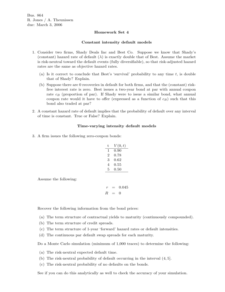
3. A firm issues the following zero-coupon bonds: t V (0 , t )
1 0 .
90
2 0 .
78
3 0 .
62
4 0 .
55
5 0 .
50
Assume the following: r = 0 .
045
R = 0
Recover the following information from the bond prices:
(a) The term structure of contractual yields to maturity (continuously compounded).
(b) The term structure of credit spreads.
(c) The term structure of 1-year ‘forward’ hazard rates or default intensities.
(d) The continuous par default swap spreads for each maturity.
Do a Monte Carlo simulation (minimum of 1,000 traces) to determine the following:
(a) The risk-neutral expected default time.
(b) The risk-neutral probability of default occurring in the interval (4 , 5].
(c) The risk-neutral probability of no defaults on the bonds.
See if you can do this analytically as well to check the accuracy of your simulation.