Hippocampal Formation Breaks Combinatorial Explosion
for Reinforcement Learning: A Conjecture
András Lőrincz
Department of Information Systems, Eötvös Loránd University
Pázmány Péter sétány 1/C
Budapest, Hungary H-1117
Abstract
There is surmounting evidence that reinforcement
learning (RL) is a good model for the dopamine system of the brain and the prefrontal cortex. RL is also
promising from the algorithmic point of view, because
recent factored RL algorithms have favorable convergence and scaling properties and can counteract the
curse of dimensionality problem, the major obstacle of
practical applications of RL methods. Learning in navigation tasks then separates (i) to the search and the encoding of the factors, such as position, direction, and
speed, and (ii) to the optimization of RL decision making by using these factors. We conjecture that the main
task of the hippocampal formation is to separate factors and encode into neocortical areas the different lowdimensional conjunctive representations of them to suit
factored RL value estimation. The mathematical framework is sketched. It includes convergent factored RL
model and autoregressive (AR) hidden process model
that finds factors including the hidden causes. The AR
model is mapped to the hippocampal formation.
Introduction
RL has been strongly motivated by psychology and neuroscience (Schultz 2002; Daw, Niv, and Dayan 2005; Delgado
2007). In addition, RL has successfully reached human level
in different games (Tesauro 1995; Conitzer and Sandholm
2007; Szita and Lőrincz 2007).We assume that reinforcement learning (RL) is the cornerstone in modeling the brain.
The core problem of RL is that learning in simple environments needs information about a number of variables,
such as the number of objects present, their shape or color,
their distances, speeds, directions, other agents, including
relatives, friends, and enemies, and so on. The state space
grows with the number of variables in the exponent. Another
source of combinatorial explosion is that the agent needs to
maintain a history of sensory information for learning and
the temporal depth multiplies the exponent. That is, RL
algorithms featuring near optimal polynomial time convergence in the number of states (Kearns and Singh 1998) are
troubled, because the state space can be exponentially large.
c 2008, Association for the Advancement of Artificial
Copyright Intelligence (www.aaai.org). All rights reserved.
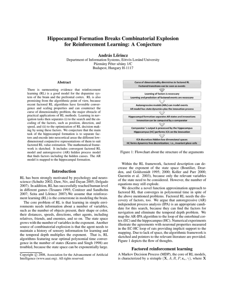
Figure 1: Flowchart about the structure of the arguments
Within the RL framework, factored description can decrease the exponent of the state space (Boutilier, Dearden, and Goldszmidt 1995; 2000; Koller and Parr 2000;
Guestrin et al. 2003), because only the relevant variables
of the state need to be considered. However, the number of
equations may still explode.
We describe a novel function approximation approach to
factored RL that converges in polynomial time in spite of
the above mentioned problems. Factored RL needs the discovery of factors, too. We argue that autoregressive (AR)
independent process analysis (IPA) is an appropriate candidate for this search, because they can find the factors for
navigation and eliminate the temporal depth problem. We
map the AR-IPA algorithm to the loop of the entorhinal cortex (EC) and the hippocampus (HC). Numerical experiments
illustrate the agreements with neuronal properties measured
in the EC-HC loop of rats providing implicit support to the
mapping. Due to lack of space, the algorithmic framework is
sketched and pointers to the relevant literature are provided.
Figure 1 depicts the flow of thoughts.
Factored reinforcement learning
A Markov Decision Process (MDP), the core of RL models,
is characterized by a sixtuple (X, A, R, P, xs , γ), where X
is a finite set of states; A is a finite set of possible actions;
R : X × A → R is the reward function of the agent, so that
R(x, a) is the reward of the agent after choosing action a in
state x; P : X × A × X → [0, 1] is the transition function
so that P (y | x, a) is the probability that the agent arrives at
state y, given that she started from x upon executing action
a; xs ∈ X is the starting state of the agent; and finally,
γ ∈ [0, 1) is the discount rate on future rewards.
A policy of the agent is a mapping π : X × A → [0, 1]
so that π(x, a) tells the probability that the agent chooses
action a in state x. For any x0 ∈ X, the policy of the agent
and the parameters of the MDP determine a stochastic process experienced by the agent through the instantiation
x0 , a0 , r0 , x1 , a1 , r1 , . . . , xt , at , rt , . . .
The goal is to find a policy that maximizes the expected
value of the discounted total reward. Let the state value
function of policy π be
∞
π
γ t rt x = x0
V (x) := E
t=0
and let the optimal value function be
V ∗ (x) := max V π (x)
π
for each x ∈ X. If V ∗ is known, it is easy to find an opti∗
mal policy π ∗ , for which V π ≡ V ∗ . Because history does
not modify transition probability distribution P (y|x, a) at
any time instant, value functions satisfy the famous Bellman
equation
P (y | x, a) R(x, a) + γV ∗ (y) . (1)
V ∗ (x) = max
a
y
Most algorithms that solve MDPs build upon some version
of the Bellman equations. For example, value can be computed by an iterative solution to the Bellman equation starting from an arbitrary value function V0 : X → R, and in
iteration t performing the update
P (y | x, a) R(x, a) + γVt (y) (2)
Vt+1 (x) := max
a
y∈X
for all x ∈ X.
Relevant results
Due to the space limitations, detailed derivations are omitted, but see the supplementary material (Szita and Lőrincz
2008). Here follows the list of the relevant facts, results, and
tasks to be accomplished.
1. MDP concepts can be generalized to factored Markov
decision processes (Boutilier, Dearden, and Goldszmidt
1995), where X is the Cartesian product of m smaller state
spaces (corresponding to individual variables):
X = X1 × X2 × . . . × Xm .
where the size of Xi is |X1 | = ni , i =
1, 2 . . . m. The size
of the full state space is N = |X| = m
i=1 ni . The number
of variables is limited by the number of factors necessary to
characterize the transition function.
2. State values, or similarly, state-action values can be
approximated by means of basis functions. In particular,
approximate value iteration with linear function approximations have attractive properties. Convergent forms can be
found in (Szita and Lőrincz 2008) and it is also shown that
these convergent forms can be carried over to case of factored value iteration.
3. Although the number of equations is still exponentially
large for the factored case, sampling methods can be exploited (Szita and Lőrincz 2008). Similarly to the results
of (Drineas, Mahoney, and Muthukrishnan 2006), the result
of sampling is that the full algorithm remains polynomial.
4. Factored RL algorithms assume that factors are already known, but in the general case, factors should be
searched for and learned. We assume that factors correspond
to hidden AR processes suggested by time discretized controlled navigation tasks. Take Newton’s equations ms̈ = F
(s: position, F : force, two dots: second temporal derivative). For short time steps, the discrete time approximation
s(t + 1) = F (t)/m − 2s(t) + s(t − 1) appears as an AR
process, but it is buried in the sensory information.
5. Factors are similar to ‘coordinates’. The direct product space of a few factors serves decision making at a time
instant and the actual factored description may change upon
each decision. RL thus needs the representation of the individual factors in order to form different conjunctive representations for evaluation from the point of view of the goals.
6. The circle is not closed yet, there are missing links.
For example, (i) AR processes may form the basis of RL
only if decisions concern the launching or the termination
of the processes. These are desired properties concerning
ongoing events, which may succeed or may not. The so
called event-based description (Szita, Takács, and Lőrincz
2003) seems appropriate for this formalization. Furthermore, (ii) different AR processes may coexist and decision
making may concern low-complexity combinations (i.e., a
small number of the processes) at a time. The appropriate
formalism, low-complexity rule based policy iteration (Szita
and Lőrincz 2007) may overcome this obstacle if it can be
extended to low-complexity AR-based policy iteration.
7. The envisioned learning sequence uncovers other missing pieces. Firstly, the factors should be uncovered and the
relevant factors should be selected. The values of turning
factors on or off should be estimated. This estimation calls
for the extension of convergence proof of the factored value
iteration method (Szita and Lőrincz 2008) to that of factored
temporal difference (TD) learning, which has shown attractive properties in numerical studies (Gyenes, Bontovics, and
Lőrincz 2008). Transition probabilities need to be estimated
in order to take advantage of linear Dyna-like algorithms
(Sutton et al. 2008) in virtual thought experiences, i.e., planning. This comes handy in goal oriented multi-agent scenarios, if novel information concerning the rewards is communicated by (at least one of) the agents.
Autoregressive processes
We are to find independent AR processes and their driving
sources. Independent component analysis (ICA) and independent subspace analysis (ISA) are the key concepts for us.
We start with a note about ICA, turn to ISA and finally to
AR processes.
Note about ICA. ICA has a peculiar but sensible property
for large number of distributed sensors when the underlying space is low dimensional. In this case, ICA minimizes
mutual information by performing an apparent discretization of the low dimensional space (Lőrincz et al. 2001;
Takács and Lőrincz 2006). This property is important for
value estimation in factored RL: ICA can provide sparse
conjunctive representations for a small number of factors.
Independent Subspace Analysis. ISA (Cardoso 1998) is
a generalization of ICA. ISA assumes that certain sources
depend on each other, but the dependent groups of sources
are independent of each other, i.e., the independent groups
are multidimensional. The ISA task has been subject of
extensive research (see, e.g., (Szabó, Póczos, and Lőrincz
2007) and the references therein). ISA is important in our
modeling for the following reasons:
8. For groups of sources that are statistically independent of other ones, characterization of the sources can be
restricted to the subspace of the variables making considerable savings in the exponent of the state space.
9. Cardoso’s observation (Cardoso 1998) that components found by ICA are entailed by single independent subspaces has received mathematical support for a limited set
of distributions (Szabó, Póczos, and Lőrincz 2007). This
observation enables effective non-combinatorial search for
independent subspaces, without a priori information about
the number of subspaces and their dimensions. Thus, the
non-combinatorial algorithm provides combinatorial gains
(Póczos et al. 2007).
ISA can be used to reveal the independent source groups
of AR processes, so we can influence the processes by interacting with the sources. Let e(t) denote the concatenated
m
vector of the source components em (t) ∈ Rde . The total diM
mension of the components is De = m=1 dm
e . We assume
that for a given m, em (t) is i.i.d. in time t, and sources em
are jointly independent, i.e., I(e1 , . . . , eM ) = 0, where I(.)
denotes the mutual information of the arguments. We shall
see that the decomposition comes for non-combinatorial
costs. First we characterize the ISA task and then we extend it to the AR identifications task.
The ISA task can be formalized as follows:
x(t) = Ae(t), where e(t) = e1 (t); . . . ; eM (t) ∈ RDe (3)
The dimension of the observation x is Dx . Assume that
Dx > De , and A ∈ RDx ×De has rank De . Then, one may
assume without any loss of generality that both the observed
(x) and the hidden (e) signals are white, i.e., decorrelated
and normalized.
We are to uncover the independent subspaces. Our task
is to find orthogonal matrix W ∈ RDe ×Dx such that
y(t) = Wx(t), y(t) = y1 (t); . . . ; yM (t) , ym =
m
[y1m ; . . . ; ydmm
] ∈ Rde , (m = 1, . . . , M ) with the condition
e
that components ym are independent. Here, yim denotes the
ith coordinate of the mth estimated subspace. This task can
be solved by means of a cost function that aims to minimize
the mutual information between components:
.
J1 (W) = I(y1 , . . . , yM ).
(4)
One can rewrite J1 (W) as follows:
M
.
J2 (W) = I(y11 , . . . , ydMM
)
−
I(y1m , . . . , ydmm
).
e
e
(5)
m=1
The first term of the r.h.s. is an ICA cost function; it aims to
minimize mutual information for all coordinates. The other
term is a kind of anti-ICA term; it maximizes mutual information within the subspaces. One may try to apply a heuristics and to optimize (5) in the following order: (i) Start by
any ’infomax’-based ICA algorithm and minimize the first
term of the r.h.s. in (5). (ii) Apply only permutations on the
coordinates to optimize the second term. Surprisingly, this
heuristics leads to the global minimum of (4) in many cases.
In other words, ICA that minimizes the first term of the r.h.s.
of (5) solves the ISA task as well, apart from grouping the
coordinates into subspaces. This feature was first observed
by Cardoso (Cardoso 1998). To what extent this heuristic
works is still an open issue. Nonetheless, we consider it as
a ‘Separation Theorem’, because for elliptically symmetric
sources and for some other distribution types one can prove
that it is rigorously true (Szabó, Póczos, and Lőrincz 2007).
Another issue concerns the computation of the second
term of the r.h.s. of (5). For subspaces em of known dimensions dm
e , multi-dimensional entropy estimations can
be applied, but these are computationally expensive. Noncombinatorial estimation of the number of components and
their respective dimensions have been developed recently
(Póczos et al. 2007).
Identification of independently driven AR processes
The generalization of the ISA task to the AR identification
task in its simplest form is this
x(t) =
s(t + 1) =
As(t),
Fs(t) + e(t),
(6)
(7)
and it can be extended to higher order AR processes, moving
average processes, integrated processes and the combinations (Szabó, Póczos, and Lőrincz 2007). The identification
algorithms can be put into Hebbian (that is neurally plausible) forms (Lőrincz, Kiszlinger, and Szirtes 2008). These
Hebbian forms pose constraints that can be used to explain
several intriguing properties of the hippocampal formation
(HF). We describe the HF and the related model below.
Model of the hippocampal formation
The relevance of the hippocampal formation. The HF
seems quite similar in mammals and it is generally considered to play crucial role in the formation of declarative memory; the memory about the representations of facts, events
or rules. After lesion, remote memories remain mostly intact but the forming of new memories about new events is
severely compromised (Squire 1992; Scoville and Milner
1957): The HF is required for the acquisition of memories
(learning or creating representations), but then it carries over
200
2
[cm]
1.5
1
0.5
0
0
200
[cm]
0
[cm]
200
Figure 2: (a): Circular maze, diameter: 2m, with a short sample
trajectory. Step size varies between 11 and 55 cm. (b): Sample
input to the loop in the form of an activity map within the maze.
Activity map is shown in arbitrary units.
0.35
0.3
Input
Decorrelated input
0.25
0.2
the information to other regions so the information can be
preserved even without the HF. It is also relevant that other
forms of learning, such as learning of procedures, or category learning remain intact after hippocampal lesion.
We consider events and facts as spatio-temporal chunks
described by factors. Factors of the events may include position, direction and speed of the animal, which together provide a crude description of the dynamical state. The rat’s
HF contains place cells (mostly) invariant to rotation, head
direction cells, which have certain, but typically weak spatial modulations. Conjunctive cells are also present in the
HF. It looks that these cell ensembles, which are located at
different regions of the HF (Sargolini et al. 2006) encode
factors for navigation, whereas the cells themselves form a
crude and soft discretization of the respective factors.
ICA model of the HF. Inspired by early ideas (Attneave
1954; Barlow 1961) ICA has been suggested to take place
in the HF (Lőrincz 1998). The idea has been improved
and extended over the years (Lőrincz and Buzsáki 2000;
Lőrincz, Szatmáry, and Szirtes 2002) and the resulting
model seems powerful enough to predict intriguing features
of this region, e.g., the independence of neuronal firing in
certain areas (Redish et al. 2001), long and tunable delays in other places (Henze, Wittner, and Buzsáki 2002) and
different functional roles for different pathways of the loop
(Kloosterman, van Haeften, and da Silva 2004).
The model is flexible and can explain certain novel findings about the rat HF (McNaughton et al. 2006). We designed computer simulations to highlight the roles and the
representations of the different parts of the HF in the model.
Numerical simulations. In our simulations1 , the ‘rat’ is
‘walking’ in a circular arena and observes distributed mixed
scent patches (Fig. 2).
Information was cumulated on the trajectories and was
analyzed by AR-IPA tools. We found that the ICA transform of temporally integrated information resemble to the
response of head direction cells. The fitted AR process produces artificial neurons that represent a low-quality grid with
conjunctive position and direction information. The neural
representation of the innovation of the AR process forms a
reasonably improved hexagonal grid and the ICA transform
of this grid brings about place cells. Results for the estimation of the innovation process are shown in Fig. 3. For other
1
For a detailed description of the simulations see the online supplementary material (Lőrincz, Kiszlinger, and Szirtes 2008).
0.15
0.1
0.05
0
27
40
53
67
80
93 107
Mean edge length [cm]
120
133
0.12
Input
Decorrelated input
0.1
0.08
0.06
0.04
0.02
0
0
10
20
30
40
50
60
70
Standard deviation of vertex angles [degree]
80
Figure 3: Position dependent input. (a-c): each column shows the
output of different decorrelating units (PCA). First row: half-wave
rectified and scaled activity maps (0: black, 1: white). Second
row: 2D autocorrelation function of the activity maps and the fitted
grids. (d-e): cumulative statistics over all grids. (d): histogram of
the mean edge length of the grids for the input set and the PCA
units. (e): histogram of the standard deviation of the vertex angles
for the input set and the PCA units. (f-g): sign corrected activity
maps of two separating (ICA) units. Response is localized. (h):
superimposed map of all ICA units demonstrating that the localized units cover the full maze. For more details, see, (Lőrincz,
Kiszlinger, and Szirtes 2008).
simulations, head direction and conjunctive representations,
see (Lőrincz, Kiszlinger, and Szirtes 2008).
The mapping of the AR-IPA process to the HF is sketched
in Fig. 4, but many of the details are omitted, including the
peculiar role of the dentate gyrus, the Hebbian learning rules
for the hidden process that require two-phase operation in
the comparator loop (Lőrincz and Szabó 2007), an important
property of the HF. For these and other details, see the supplementary material (Lőrincz, Kiszlinger, and Szirtes 2008).
In sum, results are promising, although the precision of
the hexagonal grid found in the numerical studies is not yet
satisfactory. It seems hard to achieve the required precision
without motion related internal measures. In addition, the
brain somehow takes motion related information apart, e.g.,
information, which is invariant to straight motion and information, which shows rotation invariance. These components are physically separated; they are encoded in different
areas. It is unclear how to separate these factors into different brain regions. In our conjecture, state of the AR process
is characterized by direction and weak spatial information,
whereas innovation represents a different factor. These factors are discretized by the ICA algorithm. It is probable that
actions, that is, control-like information play a role in the
forming of the representations. Also, the complementarity
of the proximal and distal afferents of the subiculum and
the CA1 subfield of the hippocampus may be necessary for
the separation of motion related factors and performing ICA
on these separated factors. These are open problems of the
model.
Conclusions
Figure 4: Hippocampal formation and the model: the factor forming structure. Factored RL estimation occurs in a separate architecture, not shown here. For the prototype of the RL architecture see,
(Szita, Gyenes, and Lőrincz 2006). (a): Main connections of hippocampus (HC) and its environment. Arrows (solid circle)denote
excitatory (mostly inhibitory) connections. HC entails the dentate
gyrus (DG), the CA1 and the CA3 subfields. Respective layers
of the entorhinal cortex (EC) are denoted by roman letters. The
DG cancels moving average processes, the echoes (Lőrincz and
Buzsáki 2000) – not discussed here. The CA1 subfield approximates the position and holds its discretization, the place cells.
The subiculum approximates head directions and holds the corresponding discretization. EC layer II holds the whitened novelty, the
hexagonal grids. Other EC layers hold conjunctive representation
of the factors of CA1 and the subiculum.(b): Connections and different representations playing a role in the numerical simulations:
x: signal from cortex, r: whitened (decorrelated and normalized)
input at EC III, m: whitened novelty (i.e., innovation) of the input at EC II, h: hidden conjunctive model at EC deep layers, q:
ICA output – the multivariate AR process – at CA1 during negative
theta phase, represented also at the subiculum, e: ICA output – the
innovation – at CA1 during positive theta phase, W: separation
matrices, V: identical copies of Ws subject to backpropagating
supervisory training, Q: whitening matrices.
We started from the necessity of RL, showed that attractive convergent polynomial learning algorithms exists provided that approximate factored representation can be found.
We have argued that factors are spatial-temporal chunks
and factored representation concerns the combination of
such chunks. In this conjecture, decision making is concerned with the transitions among sets of factors, alike to
the method described in (Szita and Lőrincz 2007).
Then the trick is to learn to separate the chunks that can be
combined later. It has been proposed that the EC-HC loop
represents an AR model with the innovation held in EC layer
II (Lőrincz and Buzsáki 2000). Recent advances on ARIPA theory (Szabó, Póczos, and Lőrincz 2007; Lőrincz and
Szabó 2007) underline the option that the HC could perform
ICA. Here, we suggested that the state and the innovation of
the AR process may form (some of the) factors for RL and
that the factors are discretized by ICA.
Numerical simulations indicate that both hexagonal grids
and place cells can be developed under suitable conditions
in the model. The same simulations also point to the need
to extend the information available for ICA by control variables. The challenge for the model is to include control values such that the precision of the hexagonal grid improves
and show the intriguing property that grids faithfully follow the distortion of the (familiar) environment (Barry et al.
2007) of grid cells when the arena is distorted.
Acknowledgement
This research has been supported by the EC FET Grant FP6502386 and EC NEST Grant FP6-043261 and Air Force
Grant FA8655-07-1-3077. Any opinions, findings and conclusions or recommendations expressed in this material are
those of the authors and do not necessarily reflect the views
of the European Commission, Air Force Office of Scientific
Research, Air Force Research Laboratory.
References
Attneave, F. 1954. Some informational aspects of visual perception. Psychol. Rev. 61:183–193.
Barlow, H. B. 1961. Sensory Communication. MIT Press, Cambridge, MA. 217–234.
Barry, C.; Hayman, R.; Burgess, N.; and Jeffery, K. J. 2007.
Experience-dependent rescaling of entorhinal grids. Nature Neurosci. 10(6):682–684.
Boutilier, C.; Dearden, R.; and Goldszmidt, M. 1995. Exploiting
structure in policy construction. In In 14th Int. Joint Conf. on
Artif. Intell., 1104–1111.
Boutilier, C.; Dearden, R.; and Goldszmidt, M. 2000. Stochastic
dynamic programming with factored representations. Artif. Intell.
121:49–107.
Cardoso, J. 1998. Multidimensional independent component
analysis. In Proc. of ICASSP, volume 4, 1941–1944.
Conitzer, V., and Sandholm, T. 2007. AWESOME: A general multiagent learning algorithm that converges in self-play and
learns a best response against stationary opponents. Machine
Learning 67:23–43.
Daw, N. D.; Niv, Y.; and Dayan, P. 2005. Uncertainty-based
competition between prefrontal and dorsolateral striatal systems
for behavioral control. Nature Neurosci. 8:1704–1711.
Delgado, M. R. 2007. Reward-related responses in the human
striatum. Ann. New York Acad. Sci. 1104:70–88.
Drineas, P.; Mahoney, M. W.; and Muthukrishnan, S. 2006. Sampling algorithms for l2 regression and applications. In Proc. 17-th
Annual SODA, 1127–1136.
Guestrin, C.; Koller, D.; Gearhart, C.; and Kanodia, N. 2003.
Generalizing plans to new environments in relational MDPs. In
18th Int. Joint Conf. on Artif. Intell.
Gyenes, V.; Bontovics, A.; and Lőrincz, A. 2008. Factored temporal difference learning in the New Ties environment. Acta Cybernetica. (in press).
Henze, D. A.; Wittner, L.; and Buzsáki, G. 2002. Single granule
cells reliably discharge targets in the hippocampal CA3 network
in vivo. Nature Neurosci. 5:790–795.
Kearns, M., and Singh, S. 1998. Near-optimal reinforcement
learning in polynomial time. In 15th Int. Conf. on Machine Learning, 260–268. San Francisco, CA: Morgan Kaufmann Publishers
Inc.
Kloosterman, F.; van Haeften, T.; and da Silva, F. H. L. 2004.
Two reentrant pathways in the hippocampal-entorhinal system.
Hippocampus 14:1026–1039.
Koller, D., and Parr, R. 2000. Policy iteration for factored mdps.
In In 16th Conf. on Uncert. Artif. Intell., 326–334.
Lőrincz, A., and Buzsáki, G. 2000. Two–phase computational model training long–term memories in the entorhinal–
hippocampal region. Ann. New York Acad. Sci. 911:83–111.
Lőrincz, A., and Szabó, Z. 2007. Neurally plausible, noncombinatorial iterative independent process analysis. Neurocomputing 70:1569–1573.
Lőrincz, A.; Szirtes, G.; Takács, B.; and Buzsáki, G. 2001. Independent component analysis of temporal sequences forms place
cells. Neurocomputing 38:769–774.
Lőrincz, A.; Kiszlinger, M.; and Szirtes, G. 2008. Model of the
hippocampal formation explains the coexistence of grid cells and
place cells. http://arxiv.org/abs/0804.3176.
Lőrincz, A.; Szatmáry, B.; and Szirtes, G. 2002. Mystery of structure and function of sensory processing areas of the neocortex: A
resolution. J. Comp. Neurosci. 13:187–205.
Lőrincz, A. 1998. Forming independent components via temporal
locking of reconstruction architectures: A functional model of the
hippocampus. Biol. Cyb. 75:37–47.
McNaughton, B. L.; Battaglia, F. P.; Jensen, O.; Moser, E. I.; and
Moser, M. 2006. Path integration and the neural basis of the
cognitive map. Nature Rev. Neuro. 7:663–678.
Póczos, B.; Szabó, Z.; Kiszlinger, M.; and Lőrincz, A. 2007.
Independent process analysis without a priori dimensional information. Lect. Notes Comp. Sci. 4666:252–259.
Redish, A. D.; Battaglia, F. P.; Chawla, M. K.; Ekstrom, A. D.;
Gerrard, J. L.; Lipa, P.; Rosenzweig, E. S.; Worley, P. F.; Guzowski, J. F.; McNaughton, B. L.; and Barnes, C. A. 2001. Independence of firing correlates of anatomically proximate hippocampal pyramidal cells. J. Neurosci. 21:1–6.
Sargolini, F.; Fyhn, M.; Hafting, T.; McNaughton, B. L.; Witter,
M. P.; Moser, M.; and Moser, E. I. 2006. Conjunctive representation of position, direction, and velocity in entorhinal cortex.
Science 312:758–762.
Schultz, W. 2002. Getting formal with dopamine and reward.
Neuron 36:241–263.
Scoville, W. B., and Milner, B. 1957. Loss of recent memory after
bilateral hippocampal lesions. J. Neurol. Neurosurg. Psychiatry
20:11–21.
Squire, L. R. 1992. Memory and hippocampus: a synthesis of
findings with rats, monkeys and humans. Psychol. Rev. 99:195–
231.
Sutton, R.; Szepesvári, C.; Geramifard, A.; and Bowling, M.
2008. Dyna-style planning with linear function approximation
and prioritized sweeping. In Uncertainty in Artifical Intelligence.
in press.
Szabó, Z.; Póczos, B.; and Lőrincz, A. 2007. Undercomplete
blind subspace deconvolution. J. Mach. Learn. Res. 8:1063–1095.
Szita, I., and Lőrincz, A. 2007. Learning to play using lowcomplexity rule-based policies: Illustrations through Ms. PacMan. J. of Artif. Intell. Res. 30:659–684.
Szita, I., and Lőrincz, A. 2008. Factored value iteration converges. http://arxiv.org/abs/0801.2069.
Szita, I.; Gyenes, V.; and Lőrincz, A. 2006. Reinforcement learning with echo state networks. Lect. Notes Comp. Sci. 4131:830–
839.
Szita, I.; Takács, B.; and Lőrincz, A. 2003. -MDPs: Learning in
varying environments. J. of Mach. Learn. Res. 3:145–174.
Takács, B., and Lőrincz, A. 2006. Independent component analysis forms place cells in realistic robot simulations. Neurocomputing 69:1249–1252.
Tesauro, G. 1995. Temporal difference learning and TD-gammon.
Communications of the ACM 38(3):58–68.