EE630 PROJECT D
SNAKE DETECTION USING FIR AND IIR FILTERS
by LGH
Updated 7-25-2013:
You will be graded on performing steps and answering questions (indicated by ?).
1. INPUT DATA
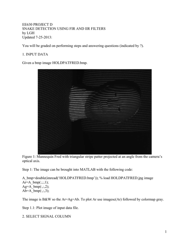
Given a bmp image HOLDPATFRED.bmp.
Figure 1: Mannequin Fred with triangular stripe patter projected at an angle from the camera’s
optical axis.
Step 1: The image can be brought into MATLAB with the following code:
A_bmp=double(imread(‘HOLDPATFRED.bmp’)); % load HOLDPATFRED.jpg image
Ar=A_bmp(:,:,1);
Ag=A_bmp(:,:,2);
Ab=A_bmp(:,:,3);
The image is B&W so the Ar=Ag=Ab. To plot Ar use imagesc(Ar) followed by colormap gray.
Step 1.1: Plot image of input data file.
2. SELECT SIGNAL COLUMN
1
Step 2.1: Select and plot, the nx column to represent a signal. Indicate which nx you used. The
size of the image is [My Nx]=size(Ar); A 1-D vector would be My by 1. sc=Ar(1:My,nx);
Figure 2: The middle column intensity of Fig. 1.
Step 2.2 DFT the 1-D signal and isolate the sine wave region. That is, determine the boundaries
of the region/s in the DFT domain that you believe represent the energy contribution of the sine
wave projection. Plot the magnitude DFT spectrum (you may suppress dc). Indicate your
boundary regions which you will be designing filters for in section 3.
3. DISCRETE TIME FILTER DESIGN
For all designs use the 1-D data in section 2 as input. Show results for each filter design in both
time and frequency domains. Remember to design a lowpass and then frequency translate it to be
a band pass filter.
3.1 Design an IIR using impulse invariance of a butterworth filter. Define your specifications and
show design process of butterworth and why you chose the specific order N?
3.2 Design an FIR using the Kaiser window. Optimize to most closely match the spectral shape
found in question 2.1?
3.3 Design an FIR using “frequency sampling approximation” of spectral region in question 2.1?
What I mean by this is take the magnitude of the spectrum that represents the striping
contribution and use it as a discrete time filter. Just window or section this region out and inverse
DFT it to get the discrete-time impulse response or just use as is in the frequency domain.
2
3.4 Choose one of the filter designs and implement on entire 2-D image. Show results in both
space and frequency domains. Take log of frequency domain to better visualize the response.
4. DFT SUBPIXEL TRANSLATION
No longer necessary
5. RECONSTRUCTION OF 3D SURFACE
Input the pattern set and G.byt files into MATLAB. Read about the mat5 format on LGH website
under software-software 3D. See appendix for MATLAB code to do this.
Let the kth frequency, nth shifted pattern image captured by the camera is represented as Ik,n(x,y)
where x and y are the column and row pixel locations, respectively. The indices are k = 0, (Nf -1)
and n = 0, 1, … (N-1) where Nf =2 and N=32. The two frequencies are kc0=1 and kc1=16.
5.1 From the pattern set decode the albedo image C.bmp, use that as the I.bmp image and obtain
the phase image YP.byt of the pattern set. To find the albedo image C.bmp, average the pattern
images together and scale between 0 and 255;
I C  x, y   I I  x, y  
1
Nf N
N f N 1
 I x, y 
k 0 n  0
(1a)
k ,n
The performance matrix I, in I.bmp, is based on the modulation amplitude [1] of the patterns
such that:
2
 N 1
  N 1

I I  x, y     I k ,n  x, y cos2n / N     I k ,n x, y sin2n / N 
 n 0
  n 0

2
(1b)
Let the k value be that of the highest frequency pattern set.
An example is shown in Fig. 5.1.
3
Figure 5.1: Average value of all captured pattern images.
The phase image for the baseline k=0 and the high frequency k=1 are determined by
 N 1

  I k ,n  x, y sin 2n / N  
 
 k  x, y   arctan  Nn 01
 I  x, y cos2n / N  
k ,n
 

n 0
(2)
For implementation, you should use atan2(y,x) instead of atan(y/x) because atan() only yields
values for 2 quadrants where as atan2() yields angles spanning all 4 quadrants. The  is added to
make the phase go from 0 to 2 rather than – to . The baseline phase is shown in Fig. 5.2 (left)
and the high frequency phase is shown in Fig. 5.2 (right).
Figure 5.2: (left) Phase k=0 and (right) phase k=1 (kc1=16).
If we take a cross section of both phase images in Fig. 5.2, we plot together, shown in Fig. 5.3,
we can see that the k=0 phase is non-ambiguous where as the k=1 is wrapped. Both vary from 0
to 2.
4
Figure 5.3: (blue) Phase k=0 cross section and (green) phase k=1 cross section.
In preparation to unwrap k=1, we normalize it by dividing by its pattern spatial frequency of kc =
16.
Figure 5.4: (blue) Phase k=0 and (green) phase k=1 divided by its projected spatial frequency of
kc1=16 cycles per FOV. Not that the slopes are very similar.
As seen in Fig. 5.4, the phase gradients of the (k=0) kc0=1 and (k=1) kc1=16 are about the same
when normalized. We need to use k=0 phase to estimate how many integer multiples of 2 to
align the k=1 phase with the k=0 phase. Once that is done, the k=0 phase is not included in the
final phase estimate, thus removing its noise contribution.
The first step [2] is to obtain the integer number of phase unwrapping wavelengths (unwrapping
cycles) that are at or below the desired value such that
 x, y   floor k c 1 0 x, y   1 x, y  / 2 
(3)
5
In units of cycles, we find the difference between the baseline phase and the unwrapping cycles
such that
r  x, y   k c 1 0  x, y    1  x, y   2   x, y  / 2
(4)
A final adjustment of +/- 1 unwrapping cycle is done by evaluating the remainder such that
  x, y   1 for r  x, y   0.5
u  x , y   
  x, y   1 for r  x, y    0.5
(5)
The final phase image is then the unwrapping cycles plus the higher frequency phase such that
  x, y   2 u  x, y    1  x, y  / k c 1
(6)
Thus, the k=1 phase is unwrapped and shown in Figs. 5.5 and 5.6.
Figure 5.5: Unwrapped phase (green) superimposed on k=0 phase.
Figure 5.6: Unwrapped phase image.
5.2 Choose a single spatial point, {x, y}, and perform DFT analysis along the temporal
dimension, n, of the pattern set, both for the base frequency and the high frequency. See if you
6
can manually estimate a correction gamma for the spatial point you chose. Show mean square
error of result (ie., generate a sine wave with estimated ,dc, amplitude, gamma and phase, then
average the sum of the square difference between the estimated and the actual). Try to choose a
point that contains a wide variation of values but does not saturate above 255. Ideally the best
point is one that varies between 0 and 255.
Assume a model of

I x , y n    x , y Ax , y  Bx , y cos 2 k c n / N   x , y   I ambient
Assume kc=1 and Iambient is the minimum value of your sequence and subtract it out such that
I x , y n   Ax' , y  Bx' , y cos 2 kc n / N   x, y 



Where  is brought in as a multiplier by A and B (ie., you don’t have to know its value). The
Gamma correction can be done after the fact by
I x, y ,corrected n  I x , y n 1/ correct
Just DFT Ix,y,corrected(n) and vary 1< correct <4 by 0.001 to minimize the harmonic error in the
DFT domain. The harmonics are where k is not equal to 2 or 32. Also, the harmonics should be
normalized such that k=2 and k=32 have the same magnitude in your model and the pixel
sequence. And k=1=dc should be zeroed out. Also note that A=B. Another approach to gamma
estimation is presented in reference [3]. From reference [3], the gamma is estimated from the
harmonics as

B1  2 B2
B1  B2
Where B1 is the first harmonic amplitude and B2 is the second harmonic amplitude. This
approach is sensitive to noise but simple to implement.
So if IA,x,y(n) is the real data and Ix,y(n) is your model data then the harmonic error is


1 31 ˆ
 I A, x , y k   Iˆx, y k 
32  3 k 3
2
 
2
2
1 ˆ

 I A, x , y 2   Iˆ A, x , y 32  
2

2
5.4 Use the G file to determine the M matrix of coefficients (we will provide this for you). A
linear triangulation paper will be provided with the assignment for explanation. Include M values
in your report.
5.5 Use the M matrix of coefficients to reconstruct the 3-D surface (we provide this MATLAB
code as well), save to mat5 format and then view in mat5 viewer. Use print screen to capture
image for this report.
7
Figure 5.7: GL3DView program displaying mat5 of Fred.
REFERENCES
1. P.S. Huang, Q. Hu, F. Jin, F.P. Chiang, “Color-encoded digital fringe projection
technique for high-speed three-dimensional surface contouring,” Optical Engineering
38(6), pp 1065-1071, (June 1999)
2. Jielin Li, L.G. Hassebrook and Chun Guan, “Optimized Two-Frequency Phase-MeasuringProfilometry Light-Sensor Temporal-Noise Sensitivity,” JOSA A, 20(1), 106-115, (2003).
3. Kai Liu, Yongchang Wang, D.L. Lau, Q. Hao and L.G. Hassebrook, “Gamma model and
its analysis for phase measuring profilometry,” JOSA A, In press, (2011).
APPENDIX: MATLAB
READ IN MAT5 (mat5read.m)
% Veeraganesh Yalla
% template script to read the
% MAT5 files
% Date: Jan 30 2004
function [xw,yw,zw,imageI,imageC] = mat5read(matfile);
% open the world coordinate
8
% files
% the x,y,z are 1-D arrays
% need to be reshaped based on
% the dimensions of I and C images
fnamex = strcat(matfile,'X.byt');fnamey = strcat(matfile,'Y.byt');
fnamez = strcat(matfile,'Z.byt');fnameC = strcat(matfile,'C.bmp');
fnameI = strcat(matfile,'I.bmp');
%
fpx = fopen(fnamex,'rb');x = fread(fpx,'float');fclose(fpx);
%
fpy = fopen(fnamey,'rb');y = fread(fpy,'float');fclose(fpy);
%
fpz = fopen(fnamez,'rb');z = fread(fpz,'float');fclose(fpz);
%open the I and C images
imageC = imread(fnameC);imageI = imread(fnameI);
%get the dimensions
[my,nx,pz] = size(imageI);
%reshape the 1D world coordinate vectors
xw = reshape(x,nx,my)';
yw = reshape(y,nx,my)';
zw = reshape(z,nx,my)';
READ IN CALIBRATION FILE *G.byt (read_calib_data.m)
%
read the calibration data
%
function needs the input calibration grid data file '.byt'
%
Npoints number of calibration points
function [coods] = read_calib_data(infname,Npoints)
%
fp = fopen(infname,'rb');
calib_data = fread(fp,'float')
fclose(fp);
%read the coordinate information
[m,n] = size(calib_data);
coods = calib_data(2:m);
coods = reshape(coods,7,Npoints)';
%
ASCII FORMAT OF calgridG.byt
Note that the data below is for a grid that has “Npoint” = 28 points. The “npoint” indicates the
last point set being edited and carries no information in itself. Each line of data or point set has 7
floating point values. Going from left to right, they are Xw, Yw, Zw, Xc, Yc, Xp, Yp where “w”
indicates a world coordinate, “c” indicates a camera coordinate and “p” indicates a projector
coordinate. Notice that Xp’s are all 0 because this is not used in the reconstruction of the 3-D data
for most applications.
Npoint=28
npoint=0
0.000000 0.000000 0.000000 937.007996 1490.270020 0.000000 4.174830
0.000000 15.875000 0.000000 935.841003 1260.900024 0.000000 3.619083
0.000000 31.750000 0.000000 934.781982 1027.890015 0.000000 3.059905
0.000000 47.625000 0.000000 933.473999 796.344971 0.000000 2.512760
15.875000 0.000000 12.700000 1178.099976 1512.079956 0.000000 3.981830
15.875000 15.875000 12.700000 1176.050049 1278.420044 0.000000 3.413457
15.875000 31.750000 12.700000 1178.459961 1040.170044 0.000000 2.843287
9
15.875000
31.750000
31.750000
31.750000
31.750000
47.625000
47.625000
47.625000
47.625000
63.500000
63.500000
63.500000
63.500000
79.375000
79.375000
79.375000
79.375000
95.250000
95.250000
95.250000
95.250000
47.625000 12.700000 1176.650024 800.879028 0.000000 2.280516
0.000000 0.000000 1397.069946 1484.609985 0.000000 4.176435
15.875000 0.000000 1397.150024 1257.400024 0.000000 3.619735
31.750000 0.000000 1396.910034 1025.890015 0.000000 3.062361
47.625000 0.000000 1396.810059 795.119995 0.000000 2.511117
0.000000 12.700000 1647.489990 1504.859985 0.000000 3.982054
15.875000 12.700000 1648.849976 1271.560059 0.000000 3.409640
31.750000 12.700000 1648.719971 1036.400024 0.000000 2.840146
47.625000 12.700000 1649.569946 800.890991 0.000000 2.282020
0.000000 0.000000 1848.689941 1479.130005 0.000000 4.177021
15.875000 0.000000 1850.829956 1252.540039 0.000000 3.619135
31.750000 0.000000 1851.040039 1023.830017 0.000000 3.064629
47.625000 0.000000 1851.250000 795.603027 0.000000 2.514975
0.000000 12.700000 2106.350098 1500.050049 0.000000 3.987183
15.875000 12.700000 2110.250000 1265.739990 0.000000 3.405886
31.750000 12.700000 2111.489990 1032.670044 0.000000 2.839072
47.625000 12.700000 2113.550049 799.932007 0.000000 2.285129
0.000000 0.000000 2292.300049 1472.890015 0.000000 4.178957
15.875000 0.000000 2294.800049 1248.540039 0.000000 3.622159
31.750000 0.000000 2297.090088 1021.719971 0.000000 3.066538
47.625000 0.000000 2300.159912 796.306030 0.000000 2.518003
WRITE IN MAT5 (mat5write.m)
function [result] = mat5write(matfile,xw,yw,zw,imageI,imageC);
% open the world coordinate files
fnamex = strcat(matfile,'X.byt');fnamey = strcat(matfile,'Y.byt');
fnamez = strcat(matfile,'Z.byt');fnameC = strcat(matfile,'C.bmp');
fnameI = strcat(matfile,'I.bmp');
%get the dimensions
[my,nx,pz] = size(imageI);
%reshape the 1D world coordinate vectors
x = reshape(xw',1,my*nx)';y = reshape(yw',1,nx*my)';z =
reshape(zw',1,nx*my)';
%xw
fpx = fopen(fnamex,'wb');fwrite(fpx,x,'float32');fclose(fpx);
%yw
fpy = fopen(fnamey,'wb');fwrite(fpy,y,'float32');fclose(fpy);
%zw
fpz = fopen(fnamez,'wb');fwrite(fpz,z,'float32');fclose(fpz);
%C
imwrite(imageC,fnameC,'bmp');imwrite(imageI,fnameI,'bmp');
%
result = 1;
10