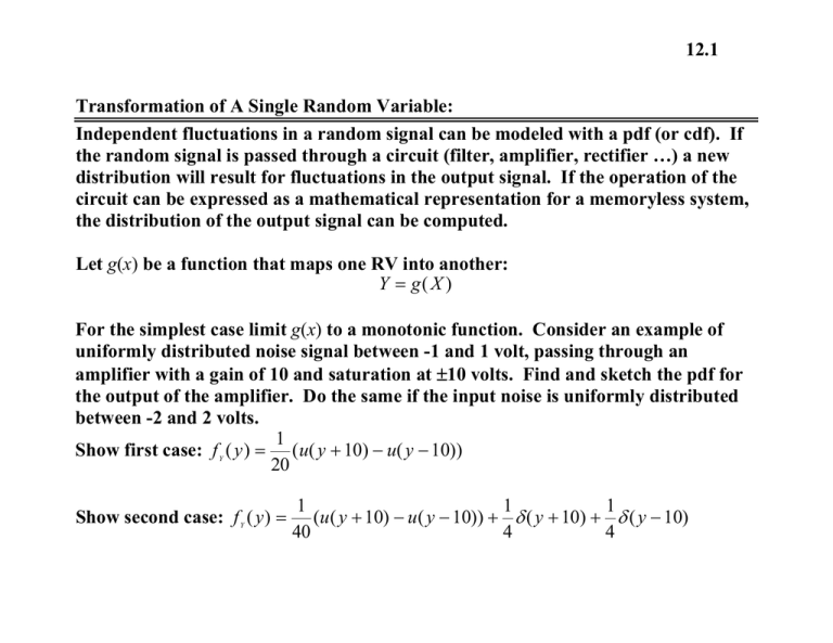
12.1
Transformation of A Single Random Variable:
Independent fluctuations in a random signal can be modeled with a pdf (or cdf). If
the random signal is passed through a circuit (filter, amplifier, rectifier …) a new
distribution will result for fluctuations in the output signal. If the operation of the
circuit can be expressed as a mathematical representation for a memoryless system,
the distribution of the output signal can be computed.
Let g(x) be a function that maps one RV into another:
Y = g( X )
For the simplest case limit g(x) to a monotonic function. Consider an example of
uniformly distributed noise signal between -1 and 1 volt, passing through an
amplifier with a gain of 10 and saturation at ±10 volts. Find and sketch the pdf for
the output of the amplifier. Do the same if the input noise is uniformly distributed
between -2 and 2 volts.
1
Show first case: f ( y ) = (u( y + 10) − u( y − 10))
20
Y
Show second case: f ( y ) =
Y
1
1
1
(u( y + 10) − u( y − 10)) + δ ( y + 10) + δ ( y − 10)
4
4
40
12.2
To obtain a process for a general transformation between continuous RVs let
y = g ( x ) where g(x0) is a monotonically increasing function, then:
F ( y ) = P(Y ≤ y ) = P[ g ( X ) ≤ g ( x )] = P ( X ≤ x ) = F ( x )
dx
Show that f ( y ) = f ( x )
dy
Likewise show if the case of a monotonically decreasing function, then:
F ( y ) = P (Y ≤ y ) = P[ g ( X ) ≥ g ( x )] = 1 − P( X ≤ x ) = 1 − F ( x )
dx
dx
For either increasing or decreasing f ( y ) = f ( x )
Show f ( y ) = − f ( x )
dy
dy
Examples: A zero mean Gaussian noise signal with an average power of .01 watts is
passed through a linear amplifier circuit with a gain of 40 dB. Find the pdf of the
noise at the output. What would the pdf be if the amp also added a bias of .5 volts?
1
⎛ y ⎞
exp⎜ −
Case 1 f ( y ) =
⎟ where σ = 10
⎝ 2σ ⎠
2π σ
0
Y
0
0
0
0
Y
0
X
0
X
x = g −1 ( y )
Y
0
0
Y
0
0
X
X
0
Y
x = g −1 ( y )
x = g −1 ( y )
2
Y
2
2
⎛ ( y − m) ⎞
exp⎜ −
Case 2 f ( y ) =
⎟
2π σ
2σ ⎠
⎝
2
1
Y
2
X
2
where σ = 10 and m = 0.5
12.3
If Y=g(X) is not monotonic, then X=g-1(Y) will not be a function. Consider Y =|X|
x=ginv(y)
10
9
8
8
6
7
4
6
2
5
0
x
y
y=g(x)
10
4
-2
3
-4
2
-6
1
-8
0
-10
-8
-6
-4
-2
0
x
2
4
6
8
10
-10
0
1
2
3
4
5
y
6
7
8
9
10
dx
does not exist. However, for the
dy
purpose for mapping one RV to another, this means that ±X is mapped into the
same Y. Therefore, nonmonotonic functions should be parsed into regions over x
where X=g-1(Y) exists as a function.
Example: A zero mean 4 watt white Gaussian signal is passed through a recitfier.
Find the distribution of the output.
−y ⎞
2
Show: f ( y ) =
exp⎛⎜
⎟ for 0 ≤ y < ∞ where σ = 2
⎝ 2σ ⎠
2π σ
Since X=g-1(Y) is not a function, the derivative
2
Y
2
2
12.4
In general, if a function is applied to a single RV Y=g(X) the distribution of a
transformed RV is computed via:
dx
f ( y) = ∑ f ( x)
where x = g ( y ), i = 1,2,3,... N is a parsing of the function
dy
into monotonic regions.
Example: An exponentially distributed RV f ( x ) = 2 exp( −2 x )u( x ) is transformed
by the function Y=(X-4)2. Find the pdf of Y.
⎧
⎛ exp(2 y ) + exp( −2 y ) ⎞
exp(
−
8
)
for 0 ≤ y < 16
⎜
⎟
⎪
y
⎝
⎠
⎪
Show: f ( y ) = ⎨
⎪exp( −8)⎛⎜ exp( −2 y ) ⎞⎟
for 16 ≤ y < ∞
⎪⎩
y
⎝
⎠
N
−1
i
Y
i =1
X
i
i
xi = gi−1 ( y )
X
Y
pdf of Y
pdf of X
0.25
2
1.8
0.2
1.6
1.4
0.15
1.2
1
0.1
0.8
0.6
0.05
0.4
0.2
0
0
0
5
10
15
X
20
25
30
0
5
10
15
Y
20
25
30