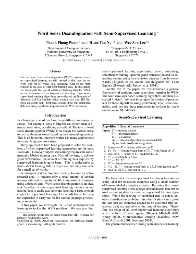
Word Sense Disambiguation with Semi-Supervised Learning ∗
Thanh Phong Pham1 and Hwee Tou Ng1,2 and Wee Sun Lee1,2
1
2
Department of Computer Science
Singapore-MIT Alliance
National University of Singapore
E4-04-10, 4 Engineering Drive 3
3 Science Drive 2, Singapore 117543
Singapore 117576
{phamthan,nght,leews}@comp.nus.edu.sg
Abstract
Current word sense disambiguation (WSD) systems based
on supervised learning are still limited in that they do not
work well for all words in a language. One of the main
reasons is the lack of sufficient training data. In this paper,
we investigate the use of unlabeled training data for WSD,
in the framework of semi-supervised learning. Four semisupervised learning algorithms are evaluated on 29 nouns of
Senseval-2 (SE2) English lexical sample task and SE2 English all-words task. Empirical results show that unlabeled
data can bring significant improvement in WSD accuracy.
semi-supervised learning algorithms, namely cotraining,
smoothed cotraining, spectral graph transduction and its cotraining variant, using the evaluation datasets from Senseval2 (SE2) English lexical sample task (Kilgarriff 2001) and
English all-words task (Palmer et al. 2001).
For the rest of the paper, we first introduce a general
framework of applying semi-supervised learning in WSD.
The four semi-supervised learning algorithms are then discussed in detail. We next investigate the choice of parameters for these algorithms using preliminary small scale evaluation, and then use those parameters to perform full scale
evaluation on SE2 datasets.
Introduction
In a language, a word can have many different meanings, or
senses. For example, bank in English can either mean a financial institution, or a sloping raised land. The task of word
sense disambiguation (WSD) is to assign the correct sense
to such ambiguous words based on the surrounding context.
This is an important problem which has many applications
in natural language processing.
Many approaches have been proposed to solve the problem, of which supervised learning approaches are the most
successful. However, supervised learning requires the use of
manually labeled training data. Most of the time, to achieve
good performance, the amount of training data required by
supervised learning is quite large. This is undesirable as
hand-labeled training data is expensive and only available
for a small set of words.
Semi-supervised learning has recently become an active
research area. It requires only a small amount of labeled
training data and is sometimes able to improve performance
using unlabeled data. Word sense disambiguation is an ideal
task for effective semi-supervised learning methods as unlabeled data is easily available and labeling a large enough
corpus for supervised learning of all words has so far been
too expensive to carry out for the natural language processing community.
In this paper, we investigate the use of semi-supervised
learning to tackle the WSD problem. We evaluate four
∗
The authors would like to thank Singapore-MIT Alliance for
partially funding this work.
c 2005, American Association for Artificial IntelliCopyright °
gence (www.aaai.org). All rights reserved.
Semi-Supervised Learning
Algorithm 1 General framework
Input: T ← training dataset
U ← unlabeled dataset
E ← test dataset
A1 ← labeling algorithm for unlabeled data
A2 ← final classification algorithm
1: feature set F ← feature selection on T
2: TF , UF ← feature vector form of T, U with feature set F
3: label set L ← labels of UF predicted by A1
4: U 0 ← add labels in L to U
5: M ← T ∪ U 0
6: F 0 ← feature selection on M
7: MF 0 , EF 0 ← feature vector form of M, E with feature set F 0
8: train A2 on MF 0 and test on EF 0
The basic idea of semi-supervised learning is to automatically label the unlabeled examples using a small number
of human labeled examples as seeds. By doing this, semisupervised learning yields a large labeled dataset that can be
used as training data for a normal supervised learning algorithm. While the labeling of unlabeled data is indeed another classification problem, this classification can exploit
the fact that all examples needed to be classified (the unlabeled data) are available at the time of training. Therefore the setup of all semi-supervised learning algorithms
is in the form of bootstrapping (Blum & Mitchell 1998;
Abney 2002), or transductive learning (Joachims 1999;
Blum & Chawla 2001; Joachims 2003).
The general framework of using semi-supervised learning
AAAI-05 / 1093
presented in this paper is shown in Algorithm 1. A1 is one of
the four semi-supervised learning algorithms which are used
to label unlabeled examples. After all these examples are labeled, we have in hand a large labeled dataset consisting of
initially human labeled seeds and the unlabeled examples
which are now labeled. This dataset is used as training data
for what we call the final classifier. In order to measure how
much improvement is obtained from using unlabeled examples, we compare the performance of the final classifier with
the baseline classifier. The baseline classifier is the same as
the final classifier, except that it is only trained on initially
labeled dataset T . In this paper, the naive Bayes algorithm
is used as the baseline and the final classifier.
Cotraining
Cotraining was first introduced in (Blum & Mitchell 1998)
as a bootstrapping method that exploits different redundant
views of data. For cotraining to work, it is sufficient that
these views are conditionally independent, and individually able to produce good classifiers. Since its first appearance, cotraining has been analyzed in different forms and
on different domains (Pierce & Cardie 2001; Abney 2002;
Mihalcea 2004). In this paper, we investigate the application of cotraining to WSD. The cotraining algorithm used,
Algorithm 2, was presented in (Pierce & Cardie 2001). This
algorithm has an advantage over the original cotraining algorithm of (Blum & Mitchell 1998) in that it tries to maintain
the sense distribution of unlabeled data to be close to that of
labeled data, and chooses only the most confidently labeled
examples instead of randomly selected examples.
Algorithm 2 Cotraining algorithm from (Pierce & Cardie
2001) maintains a data pool U 0 of size u, and labels g instances per iteration selected according to the sense distribution DL of the original labeled dataset L. U is the unlabeled
data set.
1: repeat
2:
train classifier h1 on view V1 of L
3:
train classifier h2 on view V2 of L
4:
transfer randomly selected examples from U to U 0 until
|U 0 | = u
5:
for h ∈ {h1 , h2 } do
6:
allow h to posit labels for all examples in U 0
7:
loop {g times}
8:
select label l at random according to DL
9:
transfer the most confidently labeled l example from
U 0 to L
10:
end loop
11:
end for
12: until done
In this paper, we do not use the pool U 0 . Instead, in each
iteration, all unlabeled examples are labeled and the most
confidently labeled examples among them are chosen to add
to the labeled dataset. The algorithm terminates when there
is no more unlabeled example. The two views for cotraining
are surrounding words and collocations (which will be explained in detail in a later section). The classifiers used are
naive Bayes classifiers for both views.
Smoothed Cotraining
The learning curve of cotraining has been observed to increase in performance and then decline (Pierce & Cardie
2001; Mihalcea 2004). Smoothed cotraining is the combination of cotraining with majority voting, introduced by
(Mihalcea 2004), and has the effect of delaying the decline
of performance. In smoothed cotraining, the label of an
unlabeled example is determined not only by the classifier
trained at the current iteration, but rather by majority voting
of the classifiers from all iterations. Algorithm 3 shows the
smoothed cotraining algorithm we use.
Algorithm 3 Smoothed cotraining algorithm
1: C1 = ∅
2: C2 = ∅
3: repeat
4:
train classifier h1 on view V1 of L
5:
train classifier h2 on view V2 of L
6:
C1 ← C1 ∪ {h1 }
7:
C2 ← C2 ∪ {h2 }
8:
transfer randomly selected examples from U to U 0 until
|U 0 | = u
9:
for C ∈ {C1 , C2 } do
10:
allow each h in C to posit labels for all examples in U 0
11:
label l of an example in U 0 is the label given by a majority
of classifiers in C
12:
confidence of label l is the average confidence of all classifiers in C that give label l
13:
loop {g times}
14:
select label l at random according to DL
15:
transfer most confidently labeled l example from U 0 to
L
16:
end loop
17:
end for
18: until done
Spectral Graph Transduction (SGT)
Spectral graph transduction is a new method in transductive
learning introduced in (Joachims 2003). Given a set of labeled and unlabeled examples, the task of SGT is to tag unlabeled examples with either −1 or +1. A nearest neighbor
graph G is constructed, with labeled and unlabeled examples as vertices, and edge weights between vertices denote
the similarity between the neighboring examples. SGT assigns labels to unlabeled examples by cutting G into two
subgraphs G− and G+ , and tags all examples corresponding to vertices in G− (G+ ) with −1 (+1). To give a good
prediction of labels for unlabeled examples, SGT chooses
the cut of G that minimizes the normalized cut cost
cut(G+ , G− )
min
→
−
y |{i : yi = 1}||{i : yi = −1}|
−
in which →
y is the prediction vector, and cut(G+ , G− ) is
the sum of the weights of all edges that cross the cut (i.e.,
edges with one end in G− and the other in G+ ). The
optimization is subjected to the following constraints: (i)
−
→
y ∈ {−1, +1}n , and (ii) labels for labeled training examples must be correct, i.e., vertices corresponding to positive (negative) labeled training examples must lie in G+
AAAI-05 / 1094
Local Collocations
+
View 1 graph
=
View 2 graph
Combined graph
Figure 1: Constructing the final graph from two view graphs. Edge
thickness represents edge weight.
(G− ). As this optimization itself is an NP-hard problem,
SGT performs approximate optimization using a spectral
graph method. SGT outperforms many traditional transductive learning methods on many datasets (Joachims 2003). As
SGT is a binary classifier, in order to use SGT to classify
a multi-sense word, we use one-vs-rest classifiers, i.e., one
SGT classifier for each sense class.
SGT-Cotraining
SGT-Cotraining is a variant of SGT which also exploits the
different redundant views of data as in the case of cotraining. The difference between SGT and SGT-Cotraining is
in the construction of the nearest neighbor graph. Instead
of directly computing the nearest neighbor graph, SGTCotraining constructs a separate graph for each view, and
combines them together to obtain the final graph, as shown
in Figure 1. Distinct edges in each view graph are copied
over with the same weight, while a common edge of both
graphs has its weight set to be the sum of the two weights
from both view graphs. As the edge weight measures
the similarity between examples, summing edge weights of
common edges in the final graph is intuitive in the sense
that if two examples are near to each other in both views,
we have stronger belief that they are near to each other in
the final graph. Building the final graph by combining the
two view graphs reduces the probability that the algorithm
is misled.
Knowledge Sources
In this paper, we use two knowledge sources for disambiguation: surrounding words and local collocations.
Surrounding Words
The knowledge source of surrounding words takes into account all single words (unigrams) in the surrounding context
of an ambiguous word. For each example, all the words in
the context text are extracted, converted into lower case, and
are replaced by their morphological roots. Words that are
stop words or do not contain at least one alphabet character
are removed. The remaining words of all training examples
are gathered and form the set B of surrounding words. Each
word in B forms one feature. For each training, test, or unlabeled example e, the feature corresponding to a word t in
B is 1 if and only if t appears in the context of e. A simple
feature selection on B is also employed. A feature in B is
retained if and only if it appears in at least M examples (M
is set to 3 in our experiments).
A local collocation of an ambiguous word w0 is an ordered sequence of words that appears in a narrow context
of w0 . For i = 1, 2, . . ., let w−i (wi ) be the i-th word to
the left (right) of w. Let Ci,j denote the local collocation
wi , . . . , wj (but with w0 excluded). Unlike the surrounding
words knowledge source, the local collocations knowledge
source only considers words that reside in the same sentence
as the ambiguous word w0 . Words in a collocation are converted to lower case, but stop words and non-alphabet words
(such as punctuation symbols) are not removed.
In this paper, we employ a set of 11 local collocations introduced in (Lee & Ng 2002): C−1,−1 , C1,1 , C−2,−2 , C2,2 ,
C−2,−1 , C−1,1 , C1,2 , C−3,−1 , C−2,1 , C−1,2 , and C1,3 . For
each collocation Ci,j , all its possible values appearing in the
training dataset are collected and form the features for that
collocation. Feature selection is also employed to remove
features appearing in less than M examples (M is set to 3 in
our experiments). For each example, if its collocation Ci,j
is c, then the feature corresponding to c is set to 1 in the
example.
Feature Vectors
Each labeled, unlabeled, or test example is represented by a
feature vector consisting of two parts, each part corresponding to a knowledge source. Based on the above representation of the two knowledge sources, feature vectors are binary (each dimension is either 0 or 1). Such binary feature
vectors are used for naive Bayes, cotraining, and smoothed
cotraining.
For SGT and SGT-Cotraining, the same feature vectors
are used, but with appropriate normalization. The similarity
metric used to measure the similarity between 2 examples
is the cosine similarity function. Since the number of surrounding words features is normally much larger than the
number of local collocations features, a standard normalization would result in the local collocations features contributing little to the similarity score, which is undesirable. Thus
each part of the feature vector is normalized separately, and
then the whole feature vector is normalized again. This gives
both knowledge sources the same weight in computing the
similarity score.
For algorithms that exploit the different views of data (i.e.,
cotraining, smoothed cotraining, and SGT-Cotraining), each
knowledge source is used as a view.
Datasets
Interest and Line
We evaluated the four semi-supervised learning algorithms
in two stages. In the first stage, experiments were conducted
on a small scale on two datasets, interest and line, with various learning parameter values for each algorithm. Based on
the experimental results on the interest and line datasets, the
best parameters for each algorithm were chosen to be used
for the second stage, in which large scale experiments on
SE2 datasets were conducted.
The interest corpus was taken from ACL/DCI TreeBank.
It consists of 2,369 examples of the noun interest tagged
AAAI-05 / 1095
with 6 LDOCE senses. The line corpus was obtained from
http://www.d.umn.edu/∼tpederse/data.html and consists of
4,146 examples of the noun line tagged with 6 W ORD N ET
senses.
Cotraining
Smoothed cotraining
SGT
SGT-Cotraining
interest
parameter
accuracy
line
parameter
accuracy
g = 150
g = 200
k = 100
k = 60
g = 100
g = 200
k = 80
k = 50
0.638
0.667
0.752
0.764
0.666
0.669
0.659
0.680
Lexical Sample Task
For SE2 lexical sample task, we only evaluated on all the 29
nouns in the task. Since only training and test datasets were
provided for each noun, unlabeled data were collected from
the British National Corpus (BNC). BNC was chosen as the
unlabeled data source since 90% of the training and test data
of SE2 nouns were extracted from this corpus. Each collected unlabeled example consists of consecutive complete
sentences containing an ambiguous word w, where w has
been tagged as a noun by an automatic part-of-speech tagger. The sentences are chosen such that w appears in the last
sentence of the example, and the number of words in each
example is approximately equal to the average number of
words in an SE2 (training or test) example. Also we make
sure that all the unlabeled data used do not overlap with any
training or test example of the SE2 dataset.
All-Words Task
For SE2 all-words task, we evaluate not only on nouns, but
also on verbs and adjectives. The test dataset of SE2 allwords task is used as test data, labeled training data are extracted from SemCor (Miller et al. 1994), and unlabeled
data are collected from the Wall Street Journal (WSJ) corpus, from year 1987 to 1992.
Among SE2 all-words task words, we only choose words
with at least 11 training examples in SemCor, at least one
unlabeled example in the WSJ corpus, and at least 2 senses
in SemCor. There are in total 402 such words (types) with
859 occurrences (tokens) to be disambiguated.
For each of the 402 words, we collect all occurrences of
that word from SemCor to be the labeled training data, and a
maximum of 3,000 examples from WSJ to be the unlabeled
data (if there are fewer than 3,000 examples, all available
examples are used). The context of an ambiguous word w is
chosen to be the three sentences around w, with w in the last
sentence.
Table 1: Best parameters of each algorithm on interest and line
datasets, and their respective accuracies.
• SGT and SGT-Cotraining: There are 3 parameters for
SGT: number of nearest neighbors k, tradeoff of wrongly
classifying training data c, and number of eigenvectors
used d. When c and d are large enough, changing these
two parameters does not have much effect on the classification of SGT (Joachims 2003), therefore we fixed c =
12,800 and d = 80. The only remaining parameter is k,
which was tried with values 10, 20, 30, 40, 50, 60, 70, 80,
90, and 100.
The best parameters of the four algorithms on interest and
line datasets and their corresponding accuracies are shown
in Table 1. The accuracies shown are the averages over 10
runs, where each run is based on randomly selected training and test sets. In this paper, accuracy is measured as the
percentage of test examples with correctly predicted senses.
For interest, the accuracy of the baseline naive Bayes
classifier trained on only the labeled training data is 0.676.
While the accuracy of cotraining and smoothed cotraining is lower than the baseline, SGT and SGT-Cotraining
show large improvement of up to 0.08 and 0.09 respectively.
For line, the baseline accuracy is 0.611, and all four algorithms show improvements, with SGT-Cotraining yielding
the largest improvement of 0.07.
The best parameter values vary with the algorithm and
the dataset under evaluation. For a specific algorithm, we
choose the parameter value that gives the highest average accuracy on interest and line datasets. The chosen parameter
values are g = 150 for cotraining, g = 200 for smoothed cotraining, k = 100 for SGT, and k = 60 for SGT-Cotraining.
These parameter values are then used to evaluate the four
algorithms on the larger scale SE2 datasets.
29 Senseval-2 Nouns
Empirical Results
Interest and Line
For each of the interest and line datasets, 75 examples are
randomly selected to be the test set. From the remaining examples, another 150 examples are selected to be the labeled
training dataset. The sizes of the training and test dataset are
chosen to be similar to those of SE2 English lexical sample
task. The remaining examples are treated as unlabeled examples. Labels are removed from unlabeled and test datasets
to ensure that the correct labels are not used during learning.
Using these datasets, the four semi-supervised learning
algorithms are evaluated with the following parameters:
• Cotraining and smoothed cotraining: The only parameter
is g, since the size u of unlabeled data pool is not used.
Values that are tried for g are 10, 20, 30, 40, 50, 100, 150,
and 200.
The evaluation was carried out on 29 nouns of SE2 English lexical sample task, using the parameter values chosen
above. For each noun, we tried to extract 3,000 examples
from the BNC to be used as the unlabeled dataset. For some
nouns, there were fewer than 3,000 unlabeled examples and
all of them were used as unlabeled data. For those nouns
with more than 3,000 examples in the BNC, 5 sets of 3,000
randomly chosen examples were selected to be 5 different
unlabeled datasets, and the accuracies were averaged over
the 5 sets.
The summary results are shown in Table 2, and the detailed accuracies and the dataset sizes of all the 29 nouns are
shown in Table 3.
The micro-average accuracy in Table 2 is the percentage
of the number of test examples of all 29 nouns with correctly predicted senses. The baseline accuracy is obtained
AAAI-05 / 1096
noun
train
art
authority
bar
bum
chair
channel
child
church
circuit
day
detention
dyke
facility
fatigue
feeling
grip
hearth
holiday
lady
material
mouth
nation
nature
post
restraint
sense
spade
stress
yew
196
184
304
92
138
145
129
128
170
289
63
58
114
85
102
102
64
62
105
140
119
75
92
157
91
107
65
79
57
Dataset size
test
unlabeled
98
92
151
45
69
73
64
64
85
145
32
28
58
43
51
51
32
31
53
69
60
37
46
79
45
53
33
39
28
3000
3000
3000
326
3000
3000
3000
3000
2842
3000
757
200
3000
394
3000
1599
319
3000
3000
3000
3000
3000
3000
3000
1269
3000
336
3000
200
baseline
cotraining
0.459
0.696
0.563
0.733
0.797
0.548
0.625
0.672
0.541
0.628
0.656
0.607
0.621
0.767
0.608
0.647
0.688
0.839
0.717
0.536
0.583
0.784
0.565
0.557
0.689
0.585
0.758
0.615
0.786
0.453
0.644
0.535
0.622
0.792
0.614
0.669
0.772
0.541
0.571
0.719
0.893
0.669
0.767
0.580
0.706
0.688
0.839
0.649
0.548
0.544
0.752
0.609
0.567
0.600
0.551
0.758
0.600
0.786
Accuracy
smoothed
0.459
0.661
0.552
0.733
0.797
0.608
0.681
0.772
0.506
0.574
0.750
0.893
0.659
0.767
0.678
0.706
0.719
0.839
0.664
0.588
0.583
0.779
0.661
0.585
0.600
0.547
0.758
0.657
0.786
SGT
SGT-Cotraining
0.537
0.643
0.554
0.733
0.791
0.617
0.622
0.675
0.588
0.673
0.750
0.893
0.548
0.767
0.674
0.686
0.625
0.832
0.702
0.461
0.620
0.795
0.656
0.567
0.578
0.596
0.758
0.626
0.786
0.512
0.633
0.580
0.756
0.794
0.666
0.672
0.722
0.576
0.633
0.781
0.893
0.541
0.767
0.663
0.765
0.719
0.839
0.702
0.478
0.586
0.784
0.635
0.501
0.689
0.611
0.818
0.656
0.786
Table 3: Dataset size and accuracy of the 29 nouns of SE2 English lexical sample task.
average
Baseline
Cotraining
Smoothed cotraining
SGT
SGT-Cotraining
0.629
0.626
0.642
0.643
0.650
t-test p-value
W ORD N ET Sense 1 Baseline
Naive Bayes Baseline
Cotraining
Smoothed cotraining
SGT
SGT-Cotraining
0.610
0.089
0.058
0.006
Table 2: Summary of micro-average accuracy and the p-value of
one-tail paired t-test comparing each semi-supervised learning algorithm against the naive Bayes baseline, on 29 nouns of the SE2
English lexical sample task.
by a naive Bayes algorithm training on only the human labeled training examples of SE2, without using any unlabeled
data. To test whether the improvements obtained by the
semi-supervised learning algorithms over the baseline are
significant, we perform one-tail paired t-test to compare the
accuracy of each semi-supervised learning algorithm against
the baseline. For each test example, if a classifier gives the
correct sense, its score is 1, otherwise its score is 0. The
score of a semi-supervised learning algorithm for each test
example is averaged over 5 runs. For each test example, the
scores of a semi-supervised learning algorithm and the baseline naive Bayes algorithm are paired, and the one-tail paired
t-test is performed. The p-values of one-tail paired t-test
comparing each semi-supervised learning algorithm against
the baseline are shown in Table 2.
Our empirical results indicate that cotraining does not outperform the baseline, but both smoothed cotraining and SGT
give higher accuracy than the baseline at the level of significance 0.10. In addition, SGT-Cotraining gives the highest
accuracy
t-test p-value
0.509
0.533
0.543
0.542
0.557
0.565
0.109
0.089
0.043
0.011
Table 4: Accuracy on 402 words (types) of SE2 English all-words
task and t-test p-values which measure the significance of each algorithm against the naive Bayes baseline.
accuracy with an average improvement of 0.021 over the
baseline, and is better than the baseline at the level of significance 0.01.
Senseval-2 All-Words Task
As a larger scale evaluation, we carried out experiments on
402 words (types) of SE2 English all-words task. The accuracies of the four semi-supervised learning algorithms are
shown in Table 4. For comparison purpose, accuracy of
the naive Bayes baseline and the baseline of always assigning W ORD N ET sense 1 are also included. The naive Bayes
baseline is obtained by training only on the human labeled
examples provided in SemCor, without using any unlabeled
data.
All the semi-supervised learning algorithms show improvements over both baselines, and the relative performance of the algorithms is consistent with that on the lexical
sample task, with SGT-Cotraining giving the best accuracy.
AAAI-05 / 1097
0.71
0.7
0.69
0.68
0.67
0.66
0.65
0.64
0.63
0.62
0.61
0.6
0.72
0.66
0.6
0.54
0.48
0.42
0.36
0.3
0.24
0.18
2 4 1 5 3 6 e 7 d c a b 9 8 10
1 2 e d 3 b c a 4 5 9 7 6 8 10
Figure 2: Performance comparison of naive Bayes (a), cotraining (b), smoothed cotraining (c), SGT (d), SGT-Cotraining (e),
against top 10 systems (1-10) of SE2 lexical sample task (left) and
all-words task (right). Our systems are marked with black bars.
Discussions
Our empirical results show that semi-supervised learning algorithms are able to exploit unlabeled data to improve WSD
accuracy. Although the accuracy improvement is not large,
it is statistically significant. In particular, SGT-Cotraining
gives the best improvement. To our knowledge, no prior research has investigated the use of SGT-Cotraining on WSD.
The previous work of (Mihalcea 2004) investigated the use
of cotraining and smoothed cotraining on WSD, but our results indicate that SGT-Cotraining gives better performance
than cotraining and smoothed cotraining.
Though SGT-Cotraining shows statistically significant
improvement over the baseline on average, the improvement is not observed uniformly on all nouns. For SE2 English lexical sample task, accuracy improvement is observed
on 18 nouns, ranging from 0.3% to 28.6%. 5 nouns have
unchanged accuracy, and 6 nouns have accuracy degraded,
ranging from 0.3% to 8%. The task of achieving uniform
improvement over all nouns is an important future research
topic.
Figure 2 shows a comparison of naive Bayes and the four
semi-supervised learning algorithms against the top 10 systems of SE2 for the lexical sample task and the all-words
task, ranked from highest to lowest performance. The performance shown is measured on the subset of words used in
this paper (29 nouns for lexical sample task, and 402 words
for all-words task). The semi-supervised methods use only
surrounding words and local collocations, fewer knowledge
sources than are typically used in supervised learning systems. Despite this, SGT-Cotraining ranks third among all
systems in the all-words task and its performance is comparable to the second best system, CNTS-Antwerp. The best
system, SMUaw, uses additional hand-labeled training data.
Hence, the performance of the best semi-supervised learning method is comparable to the best supervised learning
method on the SE2 all words task. However, in the lexical
sample task, semi-supervised learning methods rank lower,
suggesting that the semi-supervised learning methods may
not be ready to compete with the best supervised learning
methods when enough training data is available.
Related Work
Semi-supervised learning has been of interest to many researchers recently. Other than the four algorithms presented
in this paper, many others have been developed, including
the EM method (Nigam et al. 2000), graph min-cut (Blum
& Chawla 2001), and random walks (Zhou & Schölkopf
2004). Semi-supervised learning algorithms have been applied to a wide variety of tasks such as text categorization
(Nigam et al. 2000), base noun phrase identification (Pierce
& Cardie 2001), and named entity classification (Collins &
Singer 1999).
Mihalcea (2004) also evaluated cotraining and smoothed
cotraining for WSD, on the 29 nouns of the SE2 English lexical sample task. She reported an improvement from 53.84%
(naive Bayes baseline) to 58.35% (smoothed cotraining).
Our results are consistent with this. However, both sets of
results are not directly comparable, since Mihalcea (2004)
did not use the official SE2 test dataset for evaluation.
Conclusion
In this paper, we have investigated the use of unlabeled training data for WSD, in the framework of semi-supervised
learning. Four semi-supervised learning algorithms have
been evaluated on 29 nouns of SE2 English lexical sample
task and 402 words of SE2 English all-words task. Empirical results show that unlabeled data can bring significant
improvement in WSD accuracy.
References
Abney, S. 2002. Bootstrapping. In ACL-2002.
Blum, A., and Chawla, S. 2001. Learning from labeled and unlabeled data using graph mincuts. In ICML-2001.
Blum, A., and Mitchell, T. 1998. Combining labeled and unlabeled data with co-training. In COLT-98.
Collins, M., and Singer, Y. 1999. Unsupervised models for named
entity classification. In EMNLP/VLC-99.
Joachims, T. 1999. Transductive inference for text classification
using support vector machines. In ICML-1999.
Joachims, T. 2003. Transductive learning via spectral graph partitioning. In ICML-2003.
Kilgarriff, A. 2001. English lexical sample task description. In
SENSEVAL-2 Workshop.
Lee, Y. K., and Ng, H. T. 2002. An empirical evaluation of
knowledge sources and learning algorithms for word sense disambiguation. In EMNLP-2002.
Mihalcea, R. 2004. Co-training and self-training for word sense
disambiguation. In CoNLL-2004.
Miller, G. A.; Chodorow, M.; Landes, S.; Leacock, C.; and
Thomas, R. G. 1994. Using a semantic concordance for sense
identification. In ARPA HLT Workshop.
Nigam, K.; McCallum, A. K.; Thrun, S.; and Mitchell, T. 2000.
Text classification from labeled and unlabeled documents using
EM. Machine Learning 39(2/3).
Palmer, M.; Fellbaum, C.; Cotton, S.; Delfs, L.; and Dang, H. T.
2001. English tasks: All-words and verb lexical sample. In
SENSEVAL-2 Workshop.
Pierce, D., and Cardie, C. 2001. Limitations of co-training for
natural language learning from large datasets. In EMNLP-2001.
Zhou, D., and Schölkopf, B. 2004. Learning from labeled and
unlabeled data using random walks. In DAGM-Symposium.
AAAI-05 / 1098