From: AAAI-96 Proceedings. Copyright © 1996, AAAI (www.aaai.org). All rights reserved.
Managing Occurrence Branching in Qualitative Simulation
Lance Tokuda
University of Texas at Austin
Department of Computer Sciences
Austin, Texas 787 12- 1188
unicron@cs.utexas.edu
Abstract
Qualitative
simulators
can produce common sense
abstractions of complex behaviors given only partial
knowledge about a system. One of the problems which
limits the applicability of qualitative simulators is the
intractable branching of successor states encountered with
model of even modest size. Some branches may be
unavoidable due to the complex nature of a system. Other
branches may be accidental results of the model chosen.
A common source of intractability
is occurrence
branching. Occurrence branching occurs when the state
transitions of two variables are unordered with respect to
each other. This paper extends the QSIM model to
distinguish between interesting occurrence branching and
uninteresting
occurrence branching. A representation,
algorithm,
and simulator
for efficiently
handling
uninteresting branching is presented.
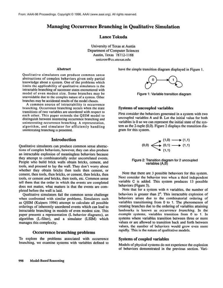
have the simple transition
diagram displayed
in Figure 1.
Figure 1: Variable transition diagram
Systems of uncoupled variables
First consider the behaviors generated in a system with two
uncoupled variables A and B. Let the initial value for both
variables is 0 so we can represent the initial state of the system as the 2-tuple (0,O). Figure 2 displays the transition diagram for this system.
Introduction
Qualitative simulators can produce common sense abstractions of complex behaviors, however, they can also produce
an intractable explosion of meaningless behaviors because
they attempt to combinatorially
order uncorrelated events.
People who build brick walls obtain bricks, cement, and
tools, and proceed to lay the wall. They don’t worry about
whether they obtain bricks then tools then cement, or
cement, then tools, then bricks, or cement, then bricks, then
tools, or cement and bricks, then tools, etc. Common sense
tell them that the order in which the events are completed
does not matter, what matters is that the events are completed before the wall is laid.
Qualitative simulators fail the common sense challenge
when confronted with similar problems. Simulators such
as QSIM (Kuipers 1994) attempt to calculate all possible
orderings of inherently unordered events which can lead to
intractable branching in models of even modest size. This
paper presents a representation
(L-behavior diagrams), an
algorithm
(L-filter),
and a simulator
(LSIM) which
manages this complexity.
Occurrence branching problems
To explore the problems
associated
with occurrence
branching, we examine systems with variables defined to
998
Model-Based Reasoning
Figure 2: Transition diagram for 2 uncoupled
variables (A,B)
Note that there are 3 possible behaviors for this system.
Next consider the behavior tree when a third independent
variable C is added. This system produces 13 possible
behaviors (Figure 3).
Note that for a system with n variables, the number of
behaviors is greater than 2”. This intractable explosion of
behaviors arises due to the combinatorial
ordering of
of
variables transitioning
from 0 to 1. The phenomenon
creating branches due to the ordering of variables attaining
landmarks
is known as occurrence branching. In the
example systems, variables transition from 0 to 1. In
systems where variables transition between three or more
values or are allowed to transition back and forth between
values, the number of behaviors would grow even more
rapidly. This is the nature of qralitative models.
Systems of couplled variables
Models of physical systems do not experience the explosion
of behaviors demonstrated in the previous section. Vari-
Next consider a double-wishbone
system composed
two wishbones connected through node A (Figure 6).
A3
of
B’
Figure 6: Double-wishbone
The number of possible behaviors
composite system is 17 (Figure 7).
resulting
from this
(0,0,0,1,0,0,1)+
(1,1,‘,‘,‘,‘,‘)
~0,0,0,0,0,0,‘
)
4
Figure 3: Transition diagram for 3 uncoupled
variables (A,B,C)
(0,0,1,0,0,0,1)-*
(l*‘,**‘***l,l)
(‘,‘,‘,‘,‘,‘,1)
ables in these models are often based on physical properties
such as position, velocity and acceleration. The velocity of
an object over time is related to both its acceleration and
position. Properties
of physical
systems are captured
through constraints. A constraint serves to prune the variable transition graph. A constraint may apply to a single
variable (e.g the variable is constant) or it may apply to
multiple variables (e.g. A = B + C).
Consider the simple model in Figure 4 which we will
refer to as a wishbone. The wishbone has four nodes
labeled A, B, C, and D.
The lines
connecting
nodes represent
constraints
between nodes. The system has the following constraints:
A is in state 1 if and only if B is in state 1.
B is in state 1 if and only if C and D are in state 1.
The wishbone can experience three possible behaviors
displayed in Figure 5.
ww,0)
b (whQl) -
(0,0,0,1,0,1,0)+
(l,l,l,l,l,l,l)
(0,0,1,0,0,1,0)-*
(l,l*l*l*l*l~l)
-E
,O)
(l,l,l,l,l,l,l)
uuwMw40,0)
(O,O,O, 1 ,O,O,O)
<
(0,0,0,1,0,0,1)+
(l,l,l,l,l,l,l)
(0,0,0,1,0,1,0)-&
(l,l,l,l,l,l,l)
(1,1,1,1.1,1,1)
Figure 7: Transition dia ram for double-wishbone
VW,W,B’, 8 ‘D’)
Figure 4: Wishbone
WL 190)-
(0,0,0,0,0,1
(1,1,1,V
(1AW
(I,l,W
Figure 5: Transition diagram for wishbone (A,B,C,D)
The wishbone exhibits traces of occurrence branching
since C can transition before, after, or at the same time as
D.
The large number of behaviors is due to occurrence
branching among variables C, D, C’, and D’. For a system
with m wishbone components (m > 1) joined at node A,
the number of behaviors is greater than 3m.
L-behavior diagrams
The C-filter algorithm employed by QSIM maintains a distinct tuple for each state of each behavior. This work proposes a compact representation which shares states among
multiple behaviors. Consider the system of two uncoupled
variables in Figure 1. The states for the behaviors of independent variables are tracked separately (Figure 8).
This representation asserts that there is no ordering specified as A and B transition from 0 to 1. Given the requirement that at least one variable must make a transition to
create a new state, Figure 8 represents the same set of
behaviors as Figure 2. Figure 9 displays the representation
for three independent variables. The cost of this representa-
Qualitative Physics
999
A
(0)__+
(1)
Figure 8: Representation for two uncoupled variables
B
A
(o)-
(1)
B
(0) ___+
(1)
W
Figure 9: Representation for three uncoupled variables
tion grows linearly with the number of variables versus the
exponential cost of the transition diagrams in Figure 2 and
Figure 3.
Next we extend this representation
to support coupled
variables.
Consider
the wishbone
from the previous
section. The system is divided into three levels (Figure 10).
0
I
\
f
OD
I
Level 1
I
Level 2
1
Level 3
Figure 11: L-behavior diagram for wishbone
uses six 4-tuples for a total of 24 variable states. The Lbehavior representation uses four 1-tuples and six 2-tuples
for a total of 16 variable
states. The L-behavior
representation
is more compact because the states for A
and B are shared for different behaviors of C and D.
Figure 12 presents a layering for the double-wishbone.
In this system there are two sets of aggregate states
produced for level 3. One set of aggregate states contains
C and D pairs and the other contains C’ and D’pairs. The
pairs are separated because they are not constrained by a
common ancestor in level 2 (i.e. they are decoupled).
Figure 10: Wishbone layering
Based on this layering, a new representation called an Lbehavior diagram is constructed. The L-behavior diagram
for a wishbone is displayed in Figure 11.
The boxes around values represent aggregate states.
Aggregate states store the behaviors of coupled variables
within the same level. The check for coupling is made
with respect to the next higher level, the current level, and
all lower levels. For the wishbone, behaviors for C and D
are placed in an aggregate state because C and D are
jointly constrained by B. The dashed lines connecting an
aggre ate state to a single state represent corresponding
states co-occur in some branch of
states f . Corresponding
the simulation. In Figure 11, the states (O,O), (O,l), and
(1,O) in cdl co-occur with state (0) in bl. The L-behavior
diagram in Figure 11 is equivalent
to the transition
diagram presented in Figure 5. The Figure 5 representation
1.QSIM states refer to a tuple which stores the value of all model
variables at a time-point or time-interval. States in this paper refer
to individual variable states or aggregate variable states - all variable values are not tracked in a single tuple.
1000
Model-Based Reasoning
/
.
,
&,pg+bJ
Figure 12: Double-wishbone layering
The L-behavior diagram for the double-wishbone
is
displayed in Figure 13.
Note that the double-wishbone
L-behavior diagram in
Figure 13 is less than twice as large as the wishbone Lbehavior diagram in Figure 11, while the double-wishbone
transition diagram in Figure 7 is approximately
six times
larger than the wishbone transition diagram in Figure 5.
The L-behavior diagram uses six I-tuples and twelve 2tuples for a total of 30 variable states. The transition
diagram in Figure 7 uses thirty-four 7-tuples for a total of
238 variable states. This is an order of magnitude
difference.
Currently,
QSIM
does
not distinguish
between
interesting and uninteresting
variables in the qualitative
model. The result is that many uninteresting
states are
calculated and displayed. Clancy was the first to address
this problem by eliminating branches off of uninteresting
variables as a post-process (Clancy & Kuipers 1993). This
solves the display problem but it does not reduce the
computational complexity of the model.
E-Filter algorithm
L-filter requires the following five elements:
1 Variable transition diagram
2 Model variables
3 Model constraints
4 Identification of interesting variables
5 Initial state of variables
(l*l)
C’,D
c’d’4
P
Figure 13: L-behavior diagram for double-wishbone
L-Filter
QSIM uses the C-filter algorithm (Kuipers 1994) to generate a behavior tree. C-filter, like the transition diagrams,
attempts to assign an ordering to all variables as they attain
landmarks. Thus, C-filter is subject to intractable occurrence branching.
L-behavior diagrams offer an implicit representation for
unordered events and avoid the problems associated with
occurrence branching. This section presents the L-filter
algorithm for efficiently computing L-behavior diagrams.
I-Branching
and U-Branching
between
interesting
occurrence
L-filter
distinguishes
branching
(I-branching)
and uninteresting
occurrence
branching (U-branching). What is interesting or uninteresting depends on the user’s perspective. The owner of a
hydraulic power plant may want to know whether the warning light flashed red before or after the dam overflowed (Ibranching). The stray dog downstream is more concerned
with its own swimming ability than the ordering of the two
events (U-branching).
L-filter is given a list of interesting variables as a part of
the system model. I-branching
is defined to be the
occurrence branching involving interesting variables. Ubranching
is defined
to be the branching
involving
uninteresting variables.
Given a system model, L-filter proceeds with the
following steps:
1 The system diagram is constructed. All variables are
identified and constraints between variables are connected with arcs (e.g. Figure 4).
2 Layering is added to the diagram. All interesting variables are placed in level 1. Other levels are identified by
performing a breadth first search. Variables at depth 1
are placed in level 2, variables at depth 2 are placed in
level 3, etc. (e.g. Figure 10). Let the number of levels be
n. The highest level refers to level 1 and the lowest level
refers to level n.
3 Aggregates within each level are identified (e.g. Figure
12). Aggregates are constructed by grouping variables
which are coupled given that variables in the next higher
level remain unchanged. ’
4 Initialize all variables and freeze all levels.
5 Set CL = lowest frozen level. Thaw(CL).
6 Advance(
ApplyConstraints(C
7 If no new states are created and CL = 1, then end the
simulation.
8 If no new states are created then goto step 5.
9 If CL < n, then Freeze(CL) and set CL = CL+l. Goto step
6.
Freeze(level) blocks any transitions
Thaw(level) removes
Freeze(level).
the
of variables in level.
transition
block
imposed
by
Advance
generates successor states for all aggregates in
level CL. The successor states are obtained by advancing
each variable in each aggregate one step in the variable
1. Two variables in level 2 may be coupled by a constraint on a
variable in level 1. For example if A = B + C where A is in level 1
and B and C are in level 2, B and C are coupled given a constant
A. For cyclic models, variables are coupled if they share a common descendant.
2. This step is analogous to running one iteration of C-filter on
level CL with the additional constraint that all variable values in
levels higher than CL do not change and all variables in lower levels are ignored.
Qualitative Physics
1001
transition diagram (see Figure
combinations are generated.
1). All possible
transition
ApplyConstraints
checks constraints among variables in
levels CL and CL-l. States which do not satisfy the constraints are pruned. If all of an aggregate’s states are deleted
then the aggregate is deleted. If all aggregates for some set
of variables corresponding
to a state are deleted, then the
state is deleted.
L-Filter applied to double-wishbone
For the double-wishbone,
the variable transition diagram,
model variables, model constraints, and initial variable values were given previously. The next step is to identify the
interesting variables. If all variables were interesting, then
the occurrence branching due to the ordering of variable
transitions
would be I-branching.
C-filter would be an
appropriate algorithm for this case since it explicitly calculates every possible ordering.
Suppose instead that the only interesting variable was A.
For this system, the ordering of variable transitions for C,
D, C’, and D’ constitutes
U-branching.
Given
this
knowledge, one would not need to unroll the L-behavior
diagram to produce all possible transition orderings. Level
1 would be the only level of interest. This is the advantage
of L-filter - I-branching is calculated explicitly while Ubranching is implicit in the representation. To illustrate the
advantage of L-filter, A is chosen as the only interesting
variable.
Given the double-wishbone
system model, L-filter
proceeds in the following steps:
Construct the system-diagram (Figure 6).
Divide the diagram into levels.
Identify aggregates within each level (Figure 12).
Set CL = 3. Thaw(3).
Advance(3). ApplyConstraints(3). This produces cdl and
c’d’l ?
Since there are no lower levels, level 3 is advanced
again. This time, no states which satisfy the constraints
are produced.
Thaw(2). Advance(2). ApplyConstraints(2). B transitions
from 0 to 1 and constraints are checked between B and
A. No states are possible since A and B must have the
same value.
Thaw( 1). Advance( 1). ApplyConstraints( 1). This produces a2. Freeze( 1).
Advance(2). ApplyConstraints(2). This produces b2 and
b’2. Freeze(2).
10 Advance(3). ApplyConstraints(3). This produces cd2,
cd3, cd4, c’d’2, c’d’3, and c’d’4.
11 Since there are no lower levels, level 3 is advanced
again. This time, no states which satisfy the constraints
are produced.
12 Thaw(2). Advance(2). ApplyConstraints(2). No new
states are possible since B is in a terminal state.
1Note that states cdl and c’d’l can be computed independently.
1002
Model-Based Reasoning
13 Thaw(l). Advance(l).
ApplyConstraints(1). No new
states are possible since A is in a terminal state. At this
point, the algorithm terminates.
The result is the L-behavior
diagram in Figure 13.
LSIM
LSIM is a simulator which uses L-filter to run QSIM models. This section discusses the changes which enable L-filter
to run on QSIM models.
Interesting variables
QSIM models specify variables, constraints, and the initial
variable state*. To apply L-filter, the QSIM model is
extended by identifying interesting variables as a part of the
model. While variables of interest to the user often represent physical properties such as distance, velocity and
acceleration, a modeler will often add abstract variables to
model the hidden complexities of a system. A problem
arises when the abstract variables create an intractable number of branches and obscure interesting behaviors.
The following scenario is commonplace
- a modeler
discovers that the simulation
is generating
too many
behaviors. The modeler introduces new variables to place
additional constraints on the system behavior. The revised
model now generates more behaviors due to occurrence
branching caused by the newly introduced variables. For
example, a user may be interested in the velocity v and
height h of a bouncing ball but the modeler may add
variables KE = K * v* and PE = L * h to model the kinetic
and potential energy of the ball. Depending on the model,
C-filter may generate more behaviors when KE and PE are
added. By identifying
v and h as the only interesting
variables, L-filter attempts to reduce the cost of Ubranching due to KE and PE by not explicitly ordering
uncoupled changes in the two variables3.
Variable transition diagrams
Variables values in QSIM are a 2-tuple consisting of a magnitude and a direction. Magnitudes transition between landmarks and intervals and directions
transition
between
increasing, steady, and decreasing. Variable transitions in
QSIM are constrained by continuity (all variables in QSIM
are continuous).
The transition of a continuous variable from a landmark
to an interval is instantaneous.
This instantaneous
change
restricts the possible transitions that other variables in
corresponding states can make. For example, if a variable
A transitions from (0,inc) to ((O,inf),inc), then a variable B
2.QIM generates all possible starting states given incomplete initial state information. L-filter assumes a single initial state but
could be extended to generate all possible starting states.
3.This would be true if KE and PE were uncoupled. A modeler is
likely to define KE + PE to be constant, thus, KE and PE would
be coupled.
in corresponding
state ((O,inf),dec) cannot transition to
(0,dec). If a variable transitions from a landmark to an
interval, then all corresponding
states in the same and
lower levels must obey the time-point to time-interval
transition rules.
When a variable transitions
from an interval to a
landmark, all corresponding
states in the same and lower
levels cannot transition from a steady value to a nonfunction
constraint).
Other
steady
value
(analytic
transitions are possible since a time-interval to time-point
transition is not instantaneous.
A set of transition rules is
given in Kuipers 1994. LSIM adds time-point and timeinterval transition rules to support continuous variables.
Other Global Constraints
QSIM has a number of global constraints which should be
detected and enforced - infinite time/infinite value, nonintersection, energy, analytic function, etc. Only the infinite
time/infinite value and the analytic function constraints are
enforced at the current time, however, L-filter does not preclude the implementation
of other global constraints.
LSIM applied to a QSIM model
The current implementation
of LSIM is severely limited
because it does not support the full complement of local
and global constraints available in QSIM. A very simple
QSIM model which exhibits occurrence branching was
chosen to illustrate that LSIM can provide an advantage
over QSIM. The system contains two objects traveling on a
line at increasing speeds in opposite directions. Branching
is introduced as the object velocities attain unevenly spaced
landmarks (Figure 14).
Constraints:
vl increasing
v2 decreasing
vl = d/dt xl
I
4
+
@
4
II
x2
4
minf
II
0
II
b
inf
Xl
xl 9
/
od
/’ ‘\
Level 1
\
Level 2
Q x2
Level 3
Figure 15: System layering
Both LSIM and QSIM are capable of producing the
desired behavior for d (d is positive and increasing). LSIM
used 28 variable states while QSIM was unable to solve
the problem with 400 5-tuples (over 2000 variable states).
When the QSIM state limit was set to 800, the simulator
consumed
over nine megabytes
of memory
before
crashing.
This example shows that LSIM can produce efficiency
gains for QSIM models. It also demonstrates
the Ubranching problem for two variables with more than two
landmarks.
Conclusions
This paper establishes the intractable nature of attempting
to order uncorrelated events. The unordered transition of
only three variables is shown to produce an order of magnitude increase in the complexity for QSIM-style systems
which use single tuples to represent system states. The Lbehavior representation distinguishes between coupled and
decoupled states is shown to be potentially more efficient
that the QSIM approach. L-filter computes L-behavior diagrams and LSIM uses L-filter and additional qualitative reasoning constraints to simulate QSIM models. For a simple
model where U-branching is prevalent, LSIM demonstrates
a two orders of magnitude benefit over QSIM.
The hope is that this work will inspire a mature version
of LSIM which supports the full complement
of QSIM
constraints
and features. LSIM can then attempt to
simulate models which where previously thought to be
intractable.
References
4----a
4
:
I
I
t
I
minf
a
b
cd
I
I
1
I
III
III
v2
0 vle
I
8
II
,I
f
g
h
inf
Figure 14: Two accelerating objects moving in
opposite directions
Kuipers, B. J., 1994. Qualitative Reasoning: Modeling and
Simulation with Incomplete Knowledge, Cambridge, MA:
MIT Press.
Clancy, D., and Kuipers, B. J. 1993. Behavior Abstraction
for Tractable Simulation. In Proceedings of the Seventh
International Workshop on Qualitative Reasoning, 57-64.
The interesting
variable is chosen to be d the
distance between the two objects. The system diagram is
displayed in Figure 15.
Qualitative Physics
1003