Massachusetts Institute of Technology
Department of Mechanical Engineering
2.003 Modeling Dynamics and Control I
Spring 2005 Prelab 3
Assigned 3/04/05, due at start of lab during week 3/07/05
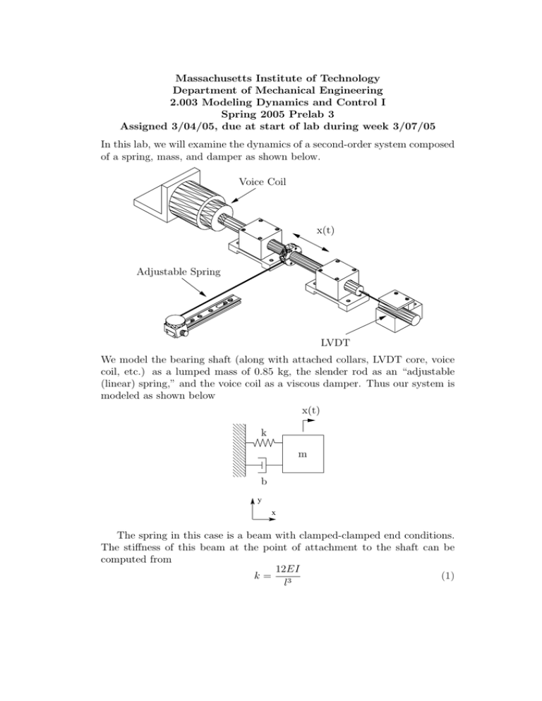
In this lab, we will examine the dynamics of a second-order system composed
of a spring, mass, and damper as shown below.
Voice Coil
x(t)
Adjustable Spring
LVDT
We model the bearing shaft (along with attached collars, LVDT core, voice
coil, etc.) as a lumped mass of 0.85 kg, the slender rod as an “adjustable
(linear) spring,” and the voice coil as a viscous damper. Thus our system is
modeled as shown below
x(t)
1
0
0
1
0
1
0
1
0
1
k
m
b
y
x
The spring in this case is a beam with clamped-clamped end conditions.
The stiffness of this beam at the point of attachment to the shaft can be
computed from
12EI
k= 3
(1)
l
2.003 Prelab 3
Assigned 3/04/2005
where
E
I
r
l
=
=
=
=
modulus of elasticity
πr4 /4
bearing shaft radius
beam length
The equation of motion for this system (Eqn. 8-9 in Ogata) is
mẍ + bẋ + kx = 0
(2)
This equation is often written in the following form (Eqn. 8-10 in Ogata)
ẍ + 2ζωn ẋ + ωn 2 x = 0
(3)
Solutions to Equation 3 can be found on pages 390-394 of Ogata. The dynam­
ics of an underdamped second-order system are often represented graphically
by plotting the system poles (or roots) in the complex plane, as shown in the
figure below.
Im{s}
s1 = −σ + j ωd
ωd = ωn 1 − ζ2
ωn
φ
−σ = −ζ ωn
Re{s}
s2 = −σ − j ωd
Figure 1: Complex roots in terms of parameters ζ, ωn , ωd , σ, and φ
�
k
= the undamped natural frequency (rad/s)
m
b
= the damping ratio
ζ = √
2 km
ωn =
2
2.003 Prelab 3
Assigned 3/04/2005
Problems
1. Given that our clamped-clamped beam has a diameter of 1.016 mm, a
modulus of elasticity of 210 GPa, and a length that can be varied from
about 50 to 160 mm, make a plot of stiffness as a function of length.
Make sure that the plot is large and accurate so that you can read off
values during lab.
2. Suppose that we’ve measured the system response shown in Figure 2.
(a) Estimate ωd and ζωn .
(b) Plot the system poles in the complex plane and use your diagram
to determine the value of ωn .
(c) Given that the mass is 0.85 kg, compute the stiffness and damping
parameters for this second-order model.
2
1.5
x(t) [cm]
1
0.5
0
−0.5
−1
−1.5
−2
0
0.5
1
1.5
Time [s]
2
2.5
3
Figure 2: Second order system response
3. Make an accurate s-plane plot showing how the poles will move as the
length of the spring rod is varied gradually from 50 to 160 mm assuming
that the voice-coil circuit is closed and we measure b = 14 N·s/m.
4. Suppose that the system is overdamped with poles at s = −3 and
s = −13 (sec−1 ). Derive expressions for the response to
(a) an initial displacement x0 with zero initial velocity
(b) an initial velocity ẋ0 with zero initial displacement
For both cases make an accurate sketch of the contribution due to each
pole as well as the total response.
5. We often wish to design a system to move from an initial to a final
position in minimum time. Assuming that the voice coil is closed and
3
2.003 Prelab 3
Assigned 3/04/2005
with the length of the spring rod anywhere from 50 to 160 mm. If the
system is released with zero velocity from a displacement of 10 mm,
determine the configuration of the system that minimizes the time that
it takes for the system to
(a) settle within 0.5 mm of equilibrium with no overshoot
(b) settle within ±1.0 mm of equilibrium if overshoot is acceptable
Use the value of b given in Problem 3 and indicate where the optimum
designs lie on your s-plane plot. Be sure to explain how you found the
optimum designs.
Matlab Hints
In questions 3 and 4, you are asked to generate a number of plots. While
you are not required to generate these using Matlab, all of these plots may
be created quickly and easily using .m files. The following functions may be
of use:
hold on holds the current plot and all axis properties so that subsequent
graphing commands add to the existing graph.
hold off returns to the default mode whereby PLOT commands erase the
previous plots and reset all axis properties before drawing new plots.
roots(c) computes the roots of the polynomial whose coefficients are the
elements of the vector c. Example:
C=[1 2 2]
A=roots(C)
Returns
A= -1+1i
-1-1i
imag(c) returns the imaginary component of a complex number c.
real(c) returns the real component of a complex number c.
length(c) returns the length of a vector c.
You may also find it useful to begin using for loops. Here is an .m file
that uses a for loop as well as the other commands.
%sample.m
a=1;
4
2.003 Prelab 3
Assigned 3/04/2005
b=2;
c=[0:1:10];
% Creates a vector from 1-10
hold on;
for i=1:length(c)
%Begins a for loop whose index starts at 1 and counts up to the size
%of c. length(c)=11 for this example
d=[a b c(i)];
%Forms d using the ith element of c
f=roots(d); %in this case 1rst element of c is 0
x=real(f); %and the 11th element is 10
y=imag(f); %d=as2 +bs+c
plot(x,y,’x’)
end
hold off
5
2.003 Prelab 3
Assigned 3/04/2005
Appendix: How an LVDT works
In this lab, we’ll use a linear variable differential transformer to measure the
shaft’s displacement. It is an electromechanical transducer that produces a
voltage proportional to the core’s displacement. It consists of (1) a movable
magnetic core, (2) primary coils, and (3) secondary coils, as shown in the
figure below.
Primary Coil
Magnetic Core
Secondary Coils
Application of an AC voltage to the primary coil induces voltages in the
two secondary coils. The voltages are opposite in polarity and proportional
to the area of overlap between the magnetized core and the secondary-coils.
When the core is centered, the voltages in the secondary coils are equal in
magnitude so they cancel out.
Figure 3 depicts a displaced magnetized core. The voltage in the top coil
increases (and the voltage in the bottom coil decreases) in proportion to the
displacement x(t), so that Vout is proportional to x(t).
Magnetized Core
Secondary Coils
x(t)
AC
Vout
Primary Coil
Figure 3: LVDT circuit
6