From: AAAI Technical Report WS-00-08. Compilation copyright © 2000, AAAI (www.aaai.org). All rights reserved.
A Constraint Model for Analyzing the Evolution of
Topological Relationships at Different Scales
Tao-Yuan Jen
Meme media Laboratory, Hokkaido University
N13W8 Kita-ku
Sapporo 060-8628, JAPAN
jenty@meme.hokudai.ac.jp
Abstract
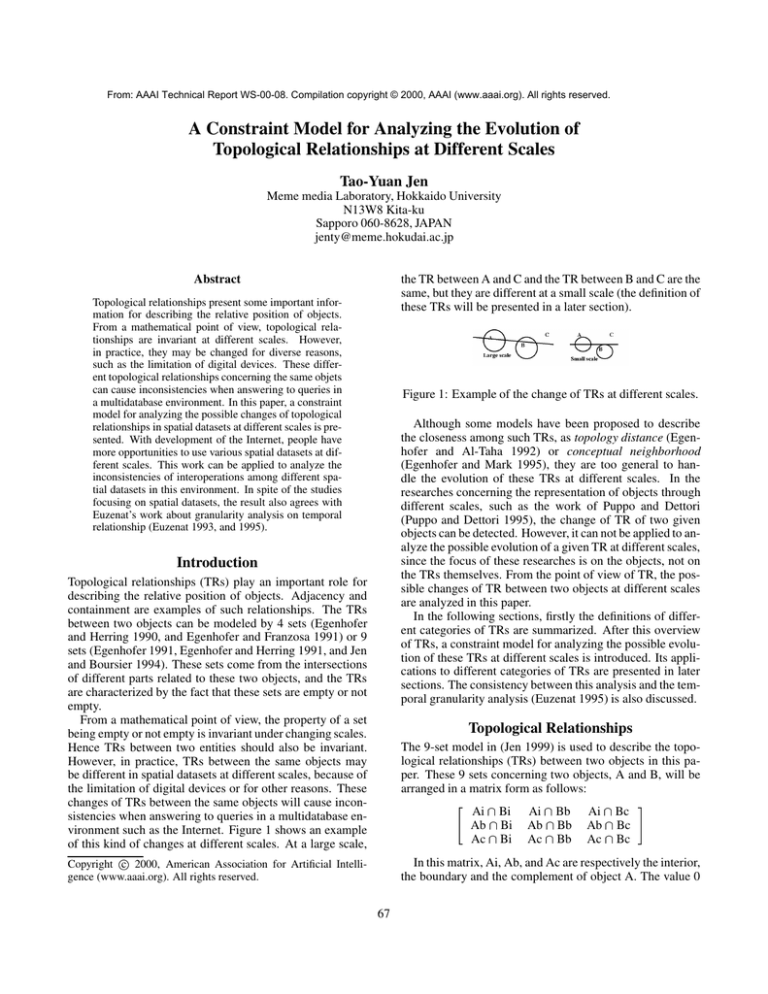
the TR between A and C and the TR between B and C are the
same, but they are different at a small scale (the definition of
these TRs will be presented in a later section).
Topological relationships present some important information for describing the relative position of objects.
From a mathematical point of view, topological relationships are invariant at different scales. However,
in practice, they may be changed for diverse reasons,
such as the limitation of digital devices. These different topological relationships concerning the same objets
can cause inconsistencies when answering to queries in
a multidatabase environment. In this paper, a constraint
model for analyzing the possible changes of topological
relationships in spatial datasets at different scales is presented. With development of the Internet, people have
more opportunities to use various spatial datasets at different scales. This work can be applied to analyze the
inconsistencies of interoperations among different spatial datasets in this environment. In spite of the studies
focusing on spatial datasets, the result also agrees with
Euzenat’s work about granularity analysis on temporal
relationship (Euzenat 1993, and 1995).
Figure 1: Example of the change of TRs at different scales.
Although some models have been proposed to describe
the closeness among such TRs, as topology distance (Egenhofer and Al-Taha 1992) or conceptual neighborhood
(Egenhofer and Mark 1995), they are too general to handle the evolution of these TRs at different scales. In the
researches concerning the representation of objects through
different scales, such as the work of Puppo and Dettori
(Puppo and Dettori 1995), the change of TR of two given
objects can be detected. However, it can not be applied to analyze the possible evolution of a given TR at different scales,
since the focus of these researches is on the objects, not on
the TRs themselves. From the point of view of TR, the possible changes of TR between two objects at different scales
are analyzed in this paper.
In the following sections, firstly the definitions of different categories of TRs are summarized. After this overview
of TRs, a constraint model for analyzing the possible evolution of these TRs at different scales is introduced. Its applications to different categories of TRs are presented in later
sections. The consistency between this analysis and the temporal granularity analysis (Euzenat 1995) is also discussed.
Introduction
Topological relationships (TRs) play an important role for
describing the relative position of objects. Adjacency and
containment are examples of such relationships. The TRs
between two objects can be modeled by 4 sets (Egenhofer
and Herring 1990, and Egenhofer and Franzosa 1991) or 9
sets (Egenhofer 1991, Egenhofer and Herring 1991, and Jen
and Boursier 1994). These sets come from the intersections
of different parts related to these two objects, and the TRs
are characterized by the fact that these sets are empty or not
empty.
From a mathematical point of view, the property of a set
being empty or not empty is invariant under changing scales.
Hence TRs between two entities should also be invariant.
However, in practice, TRs between the same objects may
be different in spatial datasets at different scales, because of
the limitation of digital devices or for other reasons. These
changes of TRs between the same objects will cause inconsistencies when answering to queries in a multidatabase environment such as the Internet. Figure 1 shows an example
of this kind of changes at different scales. At a large scale,
Topological Relationships
The 9-set model in (Jen 1999) is used to describe the topological relationships (TRs) between two objects in this paper. These 9 sets concerning two objects, A and B, will be
arranged in a matrix form as follows:
Ai
Ab
Ac
­
Bi
Bi
Bi
Ai
Ab
Ac
Bb
Bb
Bb
Ai
Ab
Ac
Bc
Bc
Bc
In this matrix, Ai, Ab, and Ac are respectively the interior,
the boundary and the complement of object A. The value 0
Copyright c 2000, American Association for Artificial Intelligence (www.aaai.org). All rights reserved.
67
will be used to indicate an empty set and the value 1 will
be represent a non-empty set. Three main categories of TRs
between two objects in Euclidean space R¾ will be presented
in ensuing sections.
TRs between two Regions
A region in this model can be seen as a disk with a finite
number of holes. The region without any hole is called simple region. The discussion in detail about these definitions
can be found in (Egenhofer and Franzosa 1991) and in (Jen
and Boursier 1994).
Figure 4: Examples of TRs between a region and a line.
TRs between two Lines
There are 33 TRs between two lines in this category. Figure
5 shows the examples of 23 TRs among them. By applying
the previously discussed interchange procedure, the examples of the other 10 TRs can be obtained.
Figure 2: Examples of TRs between two regions.
There are 18 valid TRs between two regions. Figure 2
shows the examples of 12 TRs with their matrix representation. The number of each TR is for convenience in later
discussion. The other 6 TRs whose representing matrix is
not symmetric are noted in the form of X.1, and their example can be obtained by interchanging the objects A and B in
the picture concerning the TR of number X. Figure 3 illustrates an example of this procedure. If the regions discussed
Figure 5: Examples of TRs between two lines.
Constraint Model
When using spatial dataset to describe the real world, a spatial dataset at a large scale generally contains more information and more precise information than a dataset of the same
zone at a small scale. These differences can provoke the
change of TR between the same objects at different scales
in practice. Figure 1 shows one example. Many small lakes
disappearing from a map after the scale decreasing to some
level is another example. In this paper, we would like to
distinguish which kind of changes of TRs can be made between two objects because of the precision and the quantity
of information at different scales. This kind of change will
be called valid evolution at different scales. Others will be
called non-valid evolution. If a non-valid evolution occurs
between two datasets at different scales, then the reason for
this inconsistency between the datasets has to be given attention. It may be related to the error in the acquisition of
data, or to the problem of data update in spatial dataset.
The work presented here focuses only on the changes
form large scale to small scale. The valid evolution in each
category of TRs will be illustrated in diagrams. The reverse
direction in these diagrams can be applied to present the
valid evolution from small scale to large scale.
Figure 3: Relationship between TR 2 and TR 2.1
are limited to simple regions, then there are only 8 TRs between them. These TRs are of number: 1, 3, 4, 5, 5.1, 7, 7.1,
and 10. Some TRs existing only if one of two regions with
holes can be distinguished in this model.
TRs between a Region and a Line
A line discussed in this model is a bend line with and only
with two endpoints. There exists 19 TRs between a region
and a line. Figure 4 shows the examples of these TRs.
The region with holes can not be distinguished by the representing matrix in this category of TRs. However, the evolution of TRs at different scales between a region with holes
and a line are not the same as that between a simple region
and a line. This difference can be well distinguished in the
analysis of this paper.
68
Transformation Concerning Changing Scale
dataset at a small scale in each category are analyzed. Some
propositions can be deduced from the above constraints to
analyze the valid evolution. These propositions are discussed in detail in (Jen 1999). In addition, this work also
contains the example of each valid evolution of TRs.
Since the disappearance of holes in a region provokes
some special situations, the cases including only simple regions will be analyzed separately.
The changes from a dataset at a large scale to another dataset
at a small scale of the same zone can be seen as a transformation between these two datasets. Before presenting this
type of transformation, the notion of the largest area of a region will be introduced first. The largest area R* of a region
Evolution of TRs between two Regions
Figure 6: Relationship between a region and its largest area.
R is the union of R and its holes. Figure 6 shows the relationship between a region and its largest area. For a simple
region, its largest area is itself.
The changes from a dataset D at a large scale to another
dataset D’ at a small scale of the same zone can be seen as
a transformation T from D to D’ satisfying the conditions as
follows:
For all regions R in D
If T(R)=r is also a region in D’, then
Begin
If p in (R*)c, then T(p) in (r*)c(r*)b;
If p in (R*)b, then T(p) in (r*)b;
If p in Ri, then T(p) in r;
For all holes H in R
If T(H)=h is a hole in r, then
Begin
If p in Hb, then T(p) in hb;
If p in Hi, then T(p) in h;
End;
Else T(H)=h is a point in r;
End.
For all line L in D
If T(L)=l is also a line in D’, then
Begin
If p in Lb, then T(p) in lb;
If p in Li, then T(p) in l;
End.
The first part of these conditions presents the constraints
concerning transforming a region R in D to a set r in D’. If r
is also a region in D’, then T sends the points in the largest
area R* of R to the point in the largest area r* of r, and the
points outside of the interior of R* to the points outside of
the interior of r*. The holes in R will be sent to either a hole
of r or a point of r. For a region R in D, if T(R) is a region
of D’, then it will be called a stable region between these
datasets under T. The second part of the conditions concerns
the transformation related to a line in D. L is a stable line if
L is a line in D and T(L) is also a line in D’. A stable object
is either a stable region or a stable line.
Figure 7: Schema of valid evolution of TRs between two
simple regions.
Figure 8: Schema of valid evolution of TRs between two
regions.
The valid evolution of TRs between two simple regions
are presented by arrow lines in Figure 7. The correspondence between the numbers and the TRs can be found in
Figure 2. Thus, AB means that the change from the TR A
to the TR B is a valid evolution under the transformation T.
It is important to note the reflexive and transitive properties
of these arrow lines, i.e. AA for all A in the diagram, and
if AB, and BC, then AC. These notations are applied
to all the following diagrams representing the valid evolution
between two objects. Figure 8 shows the valid evolution of
TRs between two regions.
Evolution of TRs between a Regions and a Line
The set of representing matrices for TRs between a line and
a region is the same as that for TRs between a line and a
simple region. We can not know whether a region is simple
from its TR representing matrix. However, the difference
of valid evolution of TRs concerning a simple region and a
line can be well distinguished in the analysis. Figure 9 and
Figure 10 show respectively the valid evolution among the
TRs between a simple region and a line and that between a
region and a line.
Evolution of TRs at Different Scales
From the viewpoint of transformation, the evolution of TRs
between two stable objects from a dataset at a large scale to a
69
Evolution of TRs between two Lines
Figure 11 shows the most complex result in the analysis: the
valid evolution of TRs between two lines.
Consistency with Temporal Granularity
In Allen’s model(Allen 1983), there are 13 temporal relations to describe the relationship between two temporal intervals. They are: equal( ), before( ), after(),
during(d), contains(di), overlaps(o), overlapped-by(oi),
meets(m), met-by(mi), starts(s), started-by(si), finishes(f),
and finished-by(fi). The granularity analysis concerning
these 13 relations has been studied in (Euzenat 1995). The
upward granularity of these relations can be represented by
the schema in Figure 12.
Figure 9: Schema of valid evolution of TRs between a simple region and a line.
Figure 12: Schema of upward granularity of Allen’s temporal relations.
If we see the temporal interval as the interval in Euclidean
space R½ , these 13 temporal relations will be regrouped in 8
relations, just as the TRs between two simple regions, by the
following map M :
M( )=M()=TR 1; M(m)=M(mi)=TR3 ;
M(o)=M(oi)=TR 10; M(s)=M(f)=TR 7;
M(si)=M(fi)=TR 7.1; M(d)=TR 5;
M(di)=TR 5.1; M( )=TR 4.
Under this transformation, Figure 12 is identical to Figure
7. It presents the consistency between these two analyses.
Figure 10: Schema of valid evolution of TRs between a region and a line.
Conclusion
Topological relationships (TRs) are important to retrieve information from spatial datasets. The changes of TRs in spatial datasets at different scales are studied in this paper. This
work can be applied to analyze the inconsistencies in a multidatabase environment, such as the Internet. In spite of the
focus on spatial dataset analysis, the result also agrees with
the studies of temporal granularity. This analysis will be
extended to the valid evolution of TRs across the different
categories in our ongoing work.
References
Due to the length limitation of this article, references are
only available upon request.
Figure 11: Schema of valid evolution of TRs between two
lines.
70