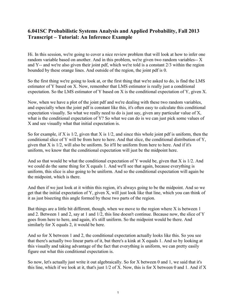
6.041SC Probabilistic Systems Analysis and Applied Probability, Fall 2013
Transcript – Tutorial: An Inference Example
Hi. In this session, we're going to cover a nice review problem that will look at how to infer one
random variable based on another. And in this problem, we're given two random variables-- X
and Y-- and we're also given their joint pdf, which we're told is a constant 2/3 within the region
bounded by these orange lines. And outside of the region, the joint pdf is 0.
So the first thing we're going to look at, or the first thing that we're asked to do, is find the LMS
estimator of Y based on X. Now, remember that LMS estimator is really just a conditional
expectation. So the LMS estimator of Y based on X is the conditional expectation of Y, given X.
Now, when we have a plot of the joint pdf and we're dealing with these two random variables,
and especially when the joint pdf is constant like this, it's often easy to calculate this conditional
expectation visually. So what we really need to do is just say, given any particular value of X,
what is the conditional expectation of Y? So what we can do is we can just pick some values of
X and see visually what that initial expectation is.
So for example, if X is 1/2, given that X is 1/2, and since this whole joint pdf is uniform, then the
conditional slice of Y will be from here to here. And that slice, the conditional distribution of Y,
given that X is 1/2, will also be uniform. So it'll be uniform from here to here. And if it's
uniform, we know that the conditional expectation will just be the midpoint here.
And so that would be what the conditional expectation of Y would be, given that X is 1/2. And
we could do the same thing for X equals 1. And we'll see that again, because everything is
uniform, this slice is also going to be uniform. And so the conditional expectation will again be
the midpoint, which is there.
And then if we just look at it within this region, it's always going to be the midpoint. And so we
get that the initial expectation of Y, given X, will just look like that line, which you can think of
it as just bisecting this angle formed by these two parts of the region.
But things are a little bit different, though, when we move to the region where X is between 1
and 2. Between 1 and 2, say at 1 and 1/2, this line doesn't continue. Because now, the slice of Y
goes from here to here, and again, it's still uniform. So the midpoint would be there. And
similarly for X equals 2, it would be here.
And so for X between 1 and 2, the conditional expectation actually looks like this. So you see
that there's actually two linear parts of it, but there's a kink at X equals 1. And so by looking at
this visually and taking advantage of the fact that everything is uniform, we can pretty easily
figure out what this conditional expectation is.
So now, let's actually just write it out algebraically. So for X between 0 and 1, we said that it's
this line, which if we look at it, that's just 1/2 of X. Now, this is for X between 0 and 1. And if X
1
is between 1 and 2, it's going to be this line, which is a slope of 1. And if we extend this down, it
hits the y-axis at negative 1/2.
So it's X minus 1/2, if X is between 1 and 2. And otherwise, it's undefined. So we'll focus on
these two cases here.
Now, the second part of the question, now that we know what the LMS estimator is, we're asked
to find what is the traditional mean squared error of this estimator? So we want to know how
good is it. And one way of capturing that is to look at the mean squared error. And so recall that
the conditional mean squared error is given by this expression.
So what we're saying is this is what we estimate Y to be. This is what y really is, so this
difference is how wrong, or the error in our estimate. We square it, because otherwise, positive
and negative errors might cancel each other out, so we square it. And then this just looking at
each individual value of x for now. So this is why it's the conditional mean squared error.
So how do we calculate this? Well, remember that this g of X, we said the LMS estimator is just
a conditional expectation. So it's just expectation of Y, given X.
Well, then if you look at this, what this reminds you of, it reminds you of the definition of what a
conditional variance is. A variance is just, you take the random variable, subtract its mean,
square it, and take the expectation of that. This is no different, except that everything is now the
conditional world of X.
So this is actually the conditional variance of Y, given X is little x. What is the conditional
variance of Y, given that X is little x? Now, we can again go back to this plot to try to help us
out.
We can split this up into regions again. So just take some little x as an example and see what the
variance is. So if little x is 1/2, then we know that the conditional distribution of Y would be
uniform, we said, from 0 up to here. Well, that point is this from 0 to 1/2.
And remember, the variance of a uniform distribution is just the width of the uniform distribution
squared, divided by 12. And so in this case, the width would be 1/2 squared over 12. And in
general, for the region of X between 0 and 1, the width of the conditional distribution of Y will
always be X, because the width will go from 0 to wherever X is. So because of that, the
conditional variance will just be X squared, the width squared, over 12, when X is between 0 and
1.
Now, let's think about the other case, where X is between 1 and 2. Well, if X is between 1 and 2,
we're over here. And now, if we take the conditional distribution of Y, it's again uniform. But the
width now, instead of varying with Y, it's always going to be the same width. Each of these
slices have the same width, and the width goes from here-- this is X minus 1, and that's X.
So if the width is always going to be a constant of 1. And so this variance is going to be 1/12.
And from that, we get our answer for the conditional mean squared error. Now, part c asks us to
2
find the mean squared error, which is given by this expression. And we'll see that it looks very
similar to this, which was the conditional mean squared error.
And now, given what we know from part b, this is easy to calculate. We can just apply total
expectation, because this is just equal to the integral of the conditional mean squared error. And
then we need to also multiply this by the pf of x, and then integrate over X. And that integral will
should be from X equals 0 to 2, because that's the only range that applies for x, given this joint
pdf.
Now, in order to do this first, though, we need to figure out what the pdf of X is. In order to do
that, we can go back to our original joint pdf of X and Y and marginalize it. So marginalizing,
you could think of it as taking this joint pdf and collapsing it onto the x-axis so that you take
everything and integrate out Y.
Now to do that, let's do that up here. We can split it up into two sections. So the section of X
between 0 and 1, we integrate the joint pdf from Y equals 0 to Y equals X, which is this portion
of this line.
So we integrate Y. The joint pdf is 2/3, and we integrate Y out from Y equals 0 to X. And then
for the portion of X from 1 to 2, we again integrate Y out. Now we integrate Y from X minus 1
up to X.
So this is X between 0 and 1, and this is X between 1 and 2. So we just do some little bit of
calculus, and we get that this is going to be 2/3 X when X is between 0 and 1. And it's going to
be 2/3 when X is between 1 and 2.
So now that we have what the marginal pdf of X is, we can plug that into this, and plug in what
we had for b, and then calculate what this actually is. So remember, we need to take care of these
two cases, these two regions-- X between 0 and 1, and X between 1 and 2.
So the conditional mean squared error for X between 0 and 1 is X squared over 2. So between 0
and 1, this first part is X squared over 12. The pdf of X in that same region is 2/3 x. And we
integrate that in the region from x equals 0 to 1.
And then, we also have the second region which is X from 1 to 2. In that region, the traditional
mean squared error from part b is 1/12. The marginal pdf of X is 2/3, and we do this integral.
And if you just carry out some calculus here, you'll get that the final answer is equal to 5/72.
Now, the last part of this question asks us, is this mean squared error the same thing-- does it
equal the expectation of the conditional variance? And it turns out that yes, it does.
And to see that, we can just take this, and use the law of iterated expectations, because iterated
expectations tells us this is in fact equal to the expectation of Y minus g of X squared, given X.
That's just applying law of iterated expectations. And then, if we look at this, this part that's
inside is exactly equal to the conditional variance of Y, given X. And so these two are, in fact,
the same.
3
In part c, we calculated what the marginal pdf of X is, and it'll actually be used later on in this
problem. So for future reference, let's just write it down here in this corner. Now, so far in this
problem, we've looked at the LMS estimator. And of course, there are other estimators that you
can use as well.
And now in part d, let's look at the linear LMS estimator. Now remember, the linear LMS
estimator is special, because it forces the estimator to have a linear relationship. So the estimator
is going to be a linear function of X.
Now, compare that to what the LMS estimator was in this case. It was two linear pieces, but
there was a kink. And so the entire estimator wasn't actually linear in X. Now, the LLMS
estimator, or the linear LMS estimator, will give us the linear estimator. It's going to be a linear
function of X.
And we know that we have a formula for this. Is the expectation of Y plus the covariance of X
and Y over the variance of X times X minus expectation of X. All right, so in order to calculate
what this is, we just need to calculate what four things are.
Now, let's start with this last one, the expected value of X. To calculate the expected value of X,
we just use a formula. And from before, we know what the pdf of X is. And so we know that this
is just going to be X times fx of x dx.
And in particular, this will give us that from 0 to 1, it's going to be X times the pdf of X is 2/3 X,
so it's 2/3 X squared. And from 1 to 2, it's going to be X times the pdf of X, which is just 2/3, so
it's 2/3 X dx. And when you calculate this out, you'll get that is equal to 11/9.
Now, let's calculate the variance of X next. In order to calculate that, let's use the formula that
variance is equal to the expectation of X squared minus the expectation of X quantity squared.
We had the expectation of X, so let's calculate what the expectation of X squared is.
Now, it's the same idea. Instead, we have X squared times f of X dx. And we'll get the same sort
of formula. We'll split it up again into two different parts from X equals 0 to X equals 1. It's
going to be X squared times pdf, so it's 2/3 X cubed dx.
And then from X equals 1 to 2, it's going to be X squared times 2/3. So it's 2/3 X squared dx.
And when we calculate this out, we'll get that it's equal to 31/18. From that, we know that the
variance is going to be equal to expectation of X squared minus expectation of X quantity
squared.
Now, expectation of X squared is 31/18. Expectation of X is 11/9. And when we calculate this,
we get that the variance is equal to 37/162.
So now we have this, and we have that. Let's calculate what expectation of Y is. Expectation of
Y, let's calculate it using the law of iterated expectations. The law of iterated expectations tells us
that this is equal to the expectation of Y conditioned on X.
4
Now, we already know what expectation of Y conditioned on X is. That was the LMS estimator
that we calculated earlier. It's this. So now we just need to calculate this out, and we can do that.
So we know that in the range from X between 0 and 1, it's equal to 1/2 X. So in the range from 0
to 1, it's equal to 1/2 X. But then, we have to use total expectation, so we have to multiply by the
pdf of X in that region which is 2/3 X dx.
And then in the range from X equals 1 to 2, this conditional expectation is X minus 1/2. And the
pdf of X in that region is 2/3. Now, when we calculate out this value, we'll get that it's equal to
7/9.
And now, the last piece is the covariance of X and Y. Remember, the covariance, we can
calculate that as the expectation of X times Y minus the expectation of X times the expectation
of Y. We already know the expectation of X and the expectation of Y, so we just need to
calculate the expectation of X times Y, the product of the two.
And for that, we'll use the definition, and we'll use the joint pdf that we have. So this is going to
be a double integral of X times Y times the joint pdf. And the tricky part here is just figuring out
what these limits are. So we'll integrate in this order-- X and Y.
Now, let's split this up. So let's focus on splitting X up. So for X between 0 and 1, we just need to
figure out what's the rate right range of Y to integrate over such that this is actually non-zero.
Because remember, the joint pdf is easy. It's just a constant 2/3. But it's only a constant 2/3
within this region.
So the difficult part is just figuring out what the limits are in order to specify that region. So for
X between 0 and 1, Y has to be between 0 and X, because this line is Y equals X. So we need to
integrate from 0 to X-- X times Y times the joint pdf, which is 2/3.
And now, let's do the other part, which is X from 1 to 2. Well, if X is from 1 to 2, in order to fall
into this region, Y has to be between X minus 1 and X. So we integrate Y from X minus 1 to X.
Against, it's X times Y times the joint pdf, which is 2/3.
And now, once we have this set up, the rest of it we can just do some calculus. And what we find
is that the final answer is equal to 41/36. Now, what that tells us is that the covariance of X and
Y, which is just expectation of X times Y, the product, minus expectation of X times expectation
of Y.
We know expectation of X times Y now. It's 41/36. Expectation of X is 11/9. Expectation of Y is
7/9. So when we substitute all of that in, we get that this covariance is 61/324.
All right, so now we have everything we need. Expectation of Y is here. Covariance is here.
Variance of X is here. And expectation of X is here. So let's substitute that in, and we can figure
out what the actual LLMS estimator is.
5
So expectation of Y we know is 7/9. Expectation of X is 11/9. And when you divide the
covariance, which is 61/324, by the variance, which is 37/162, we'll get 61/74. And so that is the
LLMS estimator that we calculated. And notice that it is, in fact, linear in X.
So let's plot that and see what it looks like. So it's going to be a line, and it's going to look like
this. So at X equals 2, it's actually a little bit below 1 and 1/2, which is what the LMS estimator
would be. At X equals 1, it's actually a little bit above 1/2, which is what the LMS estimator
would be. And then it crosses 0 around roughly 1/4, and it drops actually below 0. So if we
connect the dots, it's going to look something like this.
So notice that it's actually not too far away from the LMS estimator here. But it doesn't have the
kink because it is a line. And note also that it actually drops below. So when X is very small, you
actually estimate negative values of Y, which is actually impossible, given the joint pdf
distribution that we're given. And that is sometimes a feature or artifact of the linear LMS
estimator, that you'll get values that don't necessarily seem to make sense.
So now that we've calculated the linear LMS estimator in part d, which is this, and the LMS
estimator in part a, which is this, we've also compared them visually. The linear LMS estimator
is the one in pink, the straight line. And the LMS estimator is the one in black with the kink.
It's an interesting question to now ask, which one of these is better? And in order to judge that,
we need to come up with some sort of criterion to compare the two with. And the one that we're
going to look at in part e is the mean squared error. Which one gives the lower mean squared
error.
And so specifically, we're going to ask ourselves which of these two estimators gives us the
smaller mean squared error? Is it the linear LMS estimator given by l of X? Or is it the LMS
estimator, given by g of X?
Now, we know that the LMS estimator is the one that actually minimizes this. The LMS
estimator is designed to minimize the mean squared error. And so we know that given any
estimator of X, this one will have the smallest mean squared error. And so the linear LMS
estimator, its mean squared error has to be at least as large as the LMS estimators.
And the last part of the question now asks us to look at a third type of estimator, which is the
MEP estimator. Now, we want to ask, why is it that we haven't been using the MEP estimator in
this problem? Well, remember what the MEP estimator does.
In this case, what we would do is it would take the conditional distribution ratio of Y given any
value of X. And then it would pick the value of Y that gives the highest value in the conditional
distribution. And that would be the MEP estimate of Y.
But the problem in this case is that if you take any slice here, so a condition on any value of X,
any of these slices, if you just take this out and look at it, it's going to be uniform. This is what
the conditional distribution of Y given X is. It's going to be uniform between 0 and X. Now,
6
what the MEP rule tells us is we're going to pick the value of Y that gives us the highest point in
this conditional distribution. You can think of it as a posterior distribution.
Now, what's the problem here? Well, every single point gives us exactly the same value for this
conditional distribution. And so there's no unique MEP rule. Every single value of Y has just the
same conditional distribution. So there's no sensible way of choosing a value based on the MEP
rule in this case.
But compare that with the LMS estimator, which is just get conditional expectation. In that case,
we can always find a conditional expectation. In this case, the conditional expectation is the
midpoint, which is X/2, just as had found in part a.
OK, so in this problem, we reviewed a bunch of different ideas in terms of inference, and we
took a joint pdf of X and Y, and we used that to calculate the LMS estimator, the linear LMS
estimator. We compared the two, and then we also looked at why in this case, the MEP estimator
doesn't really make sense.
All right, so I hope that was helpful, and we'll see you next time.
7
MIT OpenCourseWare
http://ocw.mit.edu
6.041SC Probabilistic Systems Analysis and Applied Probability
Fall 2013
For information about citing these materials or our Terms of Use, visit: http://ocw.mit.edu/terms.