2.997 Decision­Making in Large­Scale Systems
MIT, Spring 2004
April 26
Handout #25
Lecture Note 21
1
Policy Search Methods
1.1
Off­Line “Unbiased” Gradient Descent Algorithm
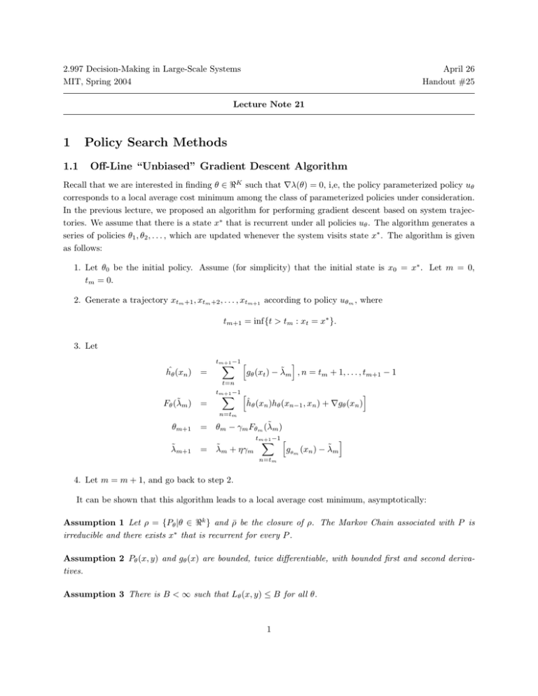
Recall that we are interested in finding θ ∈ �K such that �λ(θ) = 0, i,e, the policy parameterized policy uθ
corresponds to a local average cost minimum among the class of parameterized policies under consideration.
In the previous lecture, we proposed an algorithm for performing gradient descent based on system trajec­
tories. We assume that there is a state x∗ that is recurrent under all policies uθ . The algorithm generates a
series of policies θ1 , θ2 , . . . , which are updated whenever the system visits state x∗ . The algorithm is given
as follows:
1. Let θ0 be the initial policy. Assume (for simplicity) that the initial state is x0 = x∗ . Let m = 0,
tm = 0.
2. Generate a trajectory xtm +1 , xtm +2 , . . . , xtm+1 according to policy uθm , where
tm+1 = inf{t > tm : xt = x∗ }.
3. Let
hˆθ (xn )
=
tm+1 −1 �
�
�
˜ m , n = tm + 1, . . . , tm+1 − 1
gθ (xt ) − λ
t=n
˜m)
Fθ (λ
=
tm+1 −1 �
�
�
ˆ θ (xn )hθ (xn−1 , xn ) + �gθ (xn )
h
n=tm
θm+1
˜ m+1
λ
˜m)
= θm − γm Fθm (λ
tm+1 −1 �
�
�
˜ m + ηγm
˜m
gθm (xn ) − λ
= λ
n=tm
4. Let m = m + 1, and go back to step 2.
It can be shown that this algorithm leads to a local average cost minimum, asymptotically:
Assumption 1 Let ρ = {Pθ |θ ∈ �k } and ρ̄ be the closure of ρ. The Markov Chain associated with P is
irreducible and there exists x∗ that is recurrent for every P .
Assumption 2 Pθ (x, y) and gθ (x) are bounded, twice differentiable, with bounded first and second deriva­
tives.
Assumption 3 There is B < ∞ such that Lθ (x, y) ≤ B for all θ.
1
Assumption 4
�∞
m=1
γm = ∞ and
�∞
m=1
2
γm
< ∞.
Theorem 1 Under Assumptions 1, 2, 3 and 4, we have
lim �λ(θm ) = 0
m→∞
w.p. 1.
Some points about the algorithm are worth notice:
˜m = λ(θm ), F̃m (λ
˜ m ) would be an unbiased estimate of the gradient �λ(θm ). However,
• If we had λ
that is not the case; we only have an estimate of λ(θm ). One way of getting around this difficulty
˜ m , so as to give enough time for λ
˜ m to
would be to update the policy θm at a much slower rate than λ
converge to λ(θm ) and generate an unbiased gradient estimate before updating the policy. However,
in the algorithm described above, both θm and λ̃m are updated at the same rate, except for a constant
factor η, and convergence is still guaranteed.
• The policy θm is updated only at visits to state x∗ . This means that the algorithm can become slow
when the system is large, and cycles between visits to x∗ are long. In the sequel, we will look at
algorithms that updated the policy at every time step.
Intuition for the proof: In order to develop some intuition for the proof of Theorem 1, we will look
at the associated deterministic ODE. We have
G(θt )
(λ(θt ) − λt )
θ̇t = −�λ(θt ) −
Eθ [T ]
λ̇t
= η(λ(θt ) − λt )
We will first argue that λt converges, which implies that λt − lambda(θt ) converges to zero. It follows that,
asymptotically, θt is updated in the direction of −�λ(θt ), and we conclude that
lim �(λ(θt )) = 0.
t→∞
The proof for the stochastic algorithm follows a similar argument. It turns out that neither the ODE or
Lyapunov function approaches apply directly, and a customized, lengthy argument must be developed. The
full proof can be found in [1].
For the convergence of λt , we discuss two cases:
(1) λ0 ≥ λ(θ0 )
In this case, we first argue that λt ≥ λ(θt ). Indeed, suppose λ0 = λ(θt0 ) for some t0 . Then either
�λ(θt0 ) = 0, and the ODE reaches an equilibrium, or λ̇(θt0 ) < 0 and λ̇t0 = 0. We conclude that
λt ≥ λ(θt ), ∀t.
From the above discussion, we conclude that λt is nonincreasing and bounded. Therefore, λt converges.
(2) λ0 < λ(θ0 )
We have two possible situations:
(i) λt < λ(θt ), ∀t
In this case, ⇒ λt is nondecreasing and bounded, therefore it converges.
(ii) λt0 = λ(θt0 ) for some t0 In this case, we are back to case (1).
We conclude that λt converges, and thus (λ(θt ) − λt ) → 0. Therefore, θ̇t → −�λ(θt ) asymptotically, and
�λ(θt ) → 0.
2
1.2
Online “Unbiased” Gradient Descent Algorithm
We now develop a version of gradient descent where the policy is updated in every time step, rather than
only at visits to state x∗ . The algorithm has the advantage of being simpler and potentially faster.
First note that Fm can be computed incrementally between visits to state x∗ :
˜
Fm (θ, λ)
tm+1 −1 �
�
=
�
ˆ θ (xn )Lθ (xn−1 , xn ) + �gθ (xn )
h
n=tm
tm+1 −1
= �gθ (x∗ ) +
� �
�
ˆ θ (xn )Lθ (xn−1 , xn ) + �gθ (xn )
h
n=tm +1
tm+1 −1
∗
= �gθ (x ) +
�
�tn+1 −1
� �
n=tm +1
tm+1 −1
= �gθ (x∗ ) +
˜ Lθ (xk−1 , xk ) + �gθ (xn )
gθ (xk ) − λ
k=n
�
�
�gθ (xn ) +
n=tm +1
tm+1 −1
= �gθ (x∗ ) +
�
�
� �
n
�
�
˜
Lθ (xk−1 , xk )(gθ (xn ) − λ)
tm +1
�
� �
�gθ (xn ) + gθ (xn ) − λ̃ zn
n=tm +1
where
zn =
n
�
Lθ (xk−1 , xk ) ⇒ zn = zn−1 + Lθ (xn−1 , xn )
k=tm +1
. This suggests the following Online Algorithm:
�
�
��
˜ k )zk
θk+1 = θk − γk �gθ (xk ) + (gθk (xk ) − λ
�
0
if xk+1 = x∗
zk+1 =
zk + Lθ (xk , xk+1 ) otherwise
Assumption 5 Let P = {Pθ : θ ∈ �k } and P̄ be the closure of P. Then there exists N0 such that,
∀(P1 , P2 , . . . , PN0 ), Pi ∈ P¯ , ∀x,
N0 �
n
�
Pl (x, x∗ ) > 0.
n=1 l=1
Assumption 6
�
γk = ∞,
�
γk2 < ∞, γk ≤ γk−1 , and
�n+t
k=n (γn
− γk ) ≤ AtP γnP for some A and P .
Theorem 2 Under Assumptions 1­6, we have
�λ(θk ) → 0,
w.p.1.
The idea behind the proof of Theorem 2 is that, due to the assumptions on the step sizes γk (Assumption
6, eventually changes in the policy θm made between two consecutive visits to state x∗ are negligible, and
the algorithm behaves very similarly to the offline version. Assumption 5 is required in order to guarantee
that the time between visits to state x∗ remains small, even as the policy is not stationary.
3
1.3
Biased Gradient Estimation
In both the offline and online “unbiased” gradient descent algorithms, the variance of the estimates depends
on the variance of the times between visits to state x∗ , which can be very large depending on the system.
˜
with smaller variance.
We now look at a different algorithm, which is aimed at developing estimates �λ(θ)
˜
=
� �λ(θ).
The decrease in variance is traded against a potential bias in the estimate, i.e., we have E�λ(θ)
Note that a small amount of bias may still be acceptable since it should suffice to have estimates that have
positive inner product with the true gradient, in order for the algorithm to converge:
˜
�E�λ(θ),
�λ(θ)� > 0.
˜
We generate one such biased estimate �λ(θ)
based on a discounted­cost approximation. Let
�∞
�
�
t
Jθ,α (x) = Eθ
α g(xt )|x0 = x
t=0
Then we have
Theorem 3
�λ(θ) = (1 − α)�πθT Jθ,α + απθT �Pθ Jθ,α
�
��
�
�α λ(θ)
Proof: We have Jθ,α = g + αPθ Jθ,α . Then
�λ(θ) = �πθT g = �πθT [Jθ,α − αPθ Jθ,α ].
T
Since πθ
= πθT P, we have
�πθT = �πθT Pθ + πθT �Pθ .
Hence,
�λ(θ)
= �πθT Jθ,α − α�πθT Pθ Jθ,α
= �πθT Jθ,α − α�πθT Jθ,α + απθT �Pθ Jθ,α
=
(1 − α)�πθT Jθ,α + απθT �Pθ Jθ,α
2
The following theorem shows that �α λ(θ) can be used as an approximation to �λ(θ), if α is reasonably
close to one.
Theorem 4 Let �α λ(θ) = απθT �Pθ Jθ,α . Then
lim �α λ(θ) = �λ(θ)
α→1
Proof: We have
Jθ,α =
λ(θ)
e + hθ + O(|1 − α|).
1−α
4
Therefore,
(1 −
α)�πθTJθ,α
=
=
�
λ(θ)
(1 −
e + hθ + O(|1 − α|)
1−α
λ(θ)
(1 − α)�πθT
e + (1 − α)�πθT (hθ + O(|1 − α|))
�
��
�
1−α
T
α)�πθ
�
→0 as α→1
= λ(θ)�πθT e + O(|1 − α|)
But πθTe = 1, we have �πθT e = 0. Therefore,
(1 − α)�πθT Jθ,α = 0 + O(|1 − α|) → 0 as α → 1.
2
ˆ
If we want to use �α λ(θ) instead of �λ(θ), a simulation­based algorithm will compute Jθ,α instead of ĥθ .
We have
2
V ar(ĥθ ) ≈ O(E[T ])
�
�
ˆ
V ar Jθ,α = O
�
and
1
(1 − α)2
�
However, using �α λ(θ), we have a bias O(E[T ](1 − α)).
Based on the previous discussion, we can generate an algorithm for estimating �α λ(θ) using the same
ideas from the offline unbiased gradient descent algorithm. Indeed, consider the following algorithm, where
the policy is held fixed:
�k+1
zk+1
1
(g(xk )zk+1 − �k )
k+1
= αzk + Lθ (xk , xk+1 )
= �k +
Then it can be shown that �k → �α λ(θ), if the policy is held fixed. The gradient estimate �k can be used
for updating the policy in an offline or online fashion, just as with the unbiased gradient descent algorithms.
Assumption 7
1. unique πθ for each θ
2. |g(xk )| ≤ B, ∀x
3. |Lθ (x, y)| ≤ B, ∀x, y
Theorem 5 Under Assumption 7, we have
lim �k → �α λ(θ),
k→∞
w.p.1.
References
[1] P. Marbach and J.N. Tsitsiklis. Simulation­based optimization of Markov reward processes. IEEE
Transactions on Automatic Control, 46(2):191–209, 2001.
5