18.336 spring 2009
lecture 11
03/12/09
Efficient Methods for Sparse Linear Systems
If spectral ⇒ FFT !
If non-spectral (FD, FE):
• elimination (direct)
• iterative → multigrid
• Krylov methods (e.g. conjugate gradients)
Elimination Methods
Solve A ·
x = b
Matlab: x = A\b
If A square, regular: can use elimination methods
�
�
A symmetric positive definite: Cholesky factorization
Otherwise:
LU factorization
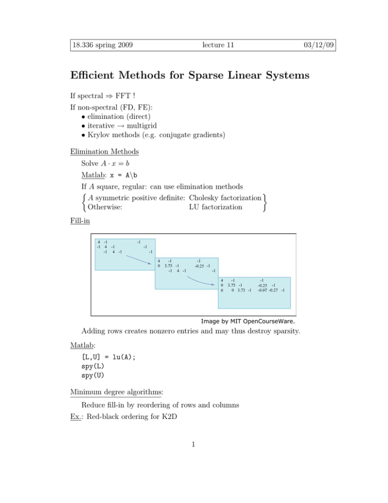
Fill-in
Image by MIT OpenCourseWare.
Adding rows creates nonzero entries and may thus destroy sparsity.
Matlab:
[L,U] = lu(A);
spy(L)
spy(U)
Minimum degree algorithms:
Reduce fill-in by reordering of rows and columns
Ex.: Red-black ordering for K2D
1
Matlab:
A non-symmetric
p = colamd(A)
[L,U] = lu(A(p,:))
Strategy: Choose remaining
column with fewest nonzeros
A symmetric
p = symamd(A)
[L,U] = lu(A(p,p))
or
[L,U] = chol(A(p,p))
Strategy: Choose remaining
meshpoint with fewest neighbors
Further:
• Graph separators
• Nested dissection
Elimination is great for small matrices whose entries are directly accessible.
Preconditioning
A ·
x = b
Condition number: κ = cond(A) = ||A|| · ||A−1 ||
|λmax |
A symmetric: cond2 (A) =
|λmin |
cond(A) � 1 ⇒ small error in b can yield large error in x
Formulate equivalent system which is better conditioned.
Left preconditioning:
solve (P −1 A) · x = P −1 b
Right preconditioning: 1. solve (AP −1 ) · y = b
2. solve P · x = b
�
�
1
1
Ex.: A =
λ ∈ {0.999, 1000.001} ⇒ cond(A) ≈ 1000
1 1000
�
�
1
0
P = diag(A) =
0 1000
cond2 (P −1 A) = cond(AP −1 ) ≈ 2.65
Image by MIT OpenCourseWare.
2
Ex.:
•P = D
•P = D + L
�
A=
Image by MIT OpenCourseWare.
• P = Lapp · Uapp (ILU = Incomplete LU factorization) [Matlab: luinc]
Iterative Methods
A·x=b
⇔ x = (I − A) · x + b
splitting
� (k+1)
�
(k)
= (I − A) · x + b
x
iteration
(0)
x
= x0
�
�
(AP −1 )y = b
Apply to precondition system:
Px = y
y (k+1) = (I − AP −1 )y (k) + b
⇔ P x(k+1) = (P − A)x(k) + b
⇔ x(k+1) = (I − P −1 A) x(k) + P −1 b
�
��
�
=M
⇔ P (x
�
(k+1)
(k)
(k)
− x ) = �b − A
��· x �
��
�
=z (k)
=r(k)
update
residual
Error:
x = A−1 b
e(k) = x − x(k)
⇒ e(k+1) = M · e(k) [independent of b ]
Iteration converges if ρ(M ) < 1
Spectral radius ρ(M ) = max |λ(M )|
Popular Preconditioners:
A=
Image by MIT OpenCourseWare.
M = I − D−1 A
M = I − (D + L)−1 A (overwrite entries
as computed)
P =D
Jacobi
P =D+L
Gauß-Seidel
P = D + wL SOR (Successive
OverRelaxation)
[better: SSOR]
3
Theorem:
�
• If A diagonal dominant
�
|aii | >
�
|aij |
⇒ Jacobi converges
j=1
�
• If Jacobi converges ⇒ Gauß-Seidel converges (× 2 faster)
• If 0 < w < 2 ⇒ SOR converges
2
�
wopt =
, µ = ρ(I − (D + I)−1 A).
2
1+ 1−µ
Multigrid
Heat Equation
ut − �2 u = f
Iterative Scheme
1
p≈ Δt
I
−→
P (u(k+1) − u(k) ) = −A ·
u(k) + f
↑
Poisson matrix
Iterative schemes behave like heat equation.
Slow convergence, fast smoothing of error.
Smoothers:
P = 23 D
Weighted Jacobi
P =D+L
Gauß Seidel
(popular)
P = D + wL SOR
(costly)
Smoother reduces high frequency error components fast.
Smooth error is rough on coarser grid.
�
�
−uxx = 1
Ex.:
u(0) = 0 = u(1)
fine grid (h = 18 )
−1
.
.
⎢
⎢ −1 . . . .
Ah = 64 ⎢
... ...
⎣
−1
−1 2
coarse grid
A2h = . . .
⎡
4
2
⎤
⎥
⎥
⎥
⎦
Interpolation: Linear
⎡
⎤
1
⎢ 2
⎥
⎢
⎥
⎢ 1 1
⎥
⎢
⎥
1⎢
7×3
2
⎥
I =
2 ⎢
⎥∈R
⎢
1 1 ⎥
⎢
⎥
⎣
2 ⎦
1
Restriction: Full Weighting
⎡
⎤
1 2 1
⎦
1 2 1
R =
14 ⎣
1 2 1
R = 12 I T
Coarse Grid Matrix:
⎡
Galerkin: A2h
⎤
2 −1
= R · Ah · I = 16 ⎣
−1 2 −1 ⎦
−1
2
5
MIT OpenCourseWare
http://ocw.mit.edu
18.336 Numerical Methods for Partial Differential Equations
Spring 2009
For information about citing these materials or our Terms of Use, visit: http://ocw.mit.edu/terms.