Time Series in Matlab
1
14.384 Time Series Analysis, Fall 2007
Recitation by Paul Schrimpf
Supplementary to lectures given by Anna Mikusheva
September 11, 2008
Recitation 2: Time Series in Matlab
Time Series in Matlab
In problem set 1, you need to estimate spectral densities and apply common filters. You
can use any software you would like, but we recommend using Matlab. It may be easier
to do simple things using more statistics oriented programs like Stata or RATs, since these
programs include pre-packaged commands for many common tasks, but you will learn more
by writing the code yourself. Also, it is generally easier to write programs for new estimators
in a full-featured programming language like Matlab’s than in the language of statistics
oriented programs. Finally, I recommend using Matlab because I happen to use Matlab, and
I will be more likely to be able to provide help if you need it.
These notes cover some slightly obscure Matlab commands that can be useful for time
series. For a more general overview, see
http://web.mit.edu/~paul_s/www/14.170/matlab.html
Disclaimer: I wrote these notes last year, and I am not entirely sure that they are com­
pletely correct. Many of the commands covered are from Matlab’s signal processing toolbox,
and they have different names and may do slightly different things than what an econometri­
cian would expect. Always read Matlab’s help and documentation before using a command.
When in doubt, double check that the command does what you think.
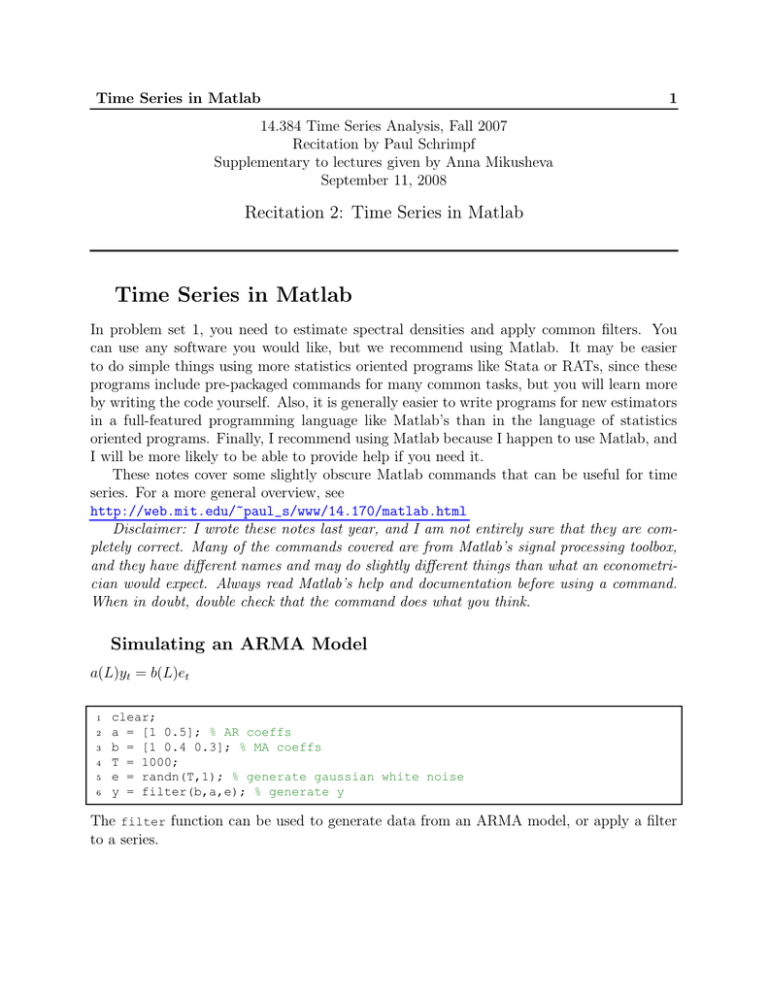
Simulating an ARMA Model
a(L)yt = b(L)et
1
2
3
4
5
6
clear;
a = [1 0.5]; % AR coeffs
b = [1 0.4 0.3]; % MA coeffs
T = 1000;
e = randn(T,1); % generate gaussian white noise
y = filter(b,a,e); % generate y
The filter function can be used to generate data from an ARMA model, or apply a filter
to a series.
Impulse-Response
2
Impulse-Response
To graph the impulse response of an ARMA, use fvtool
1
2
% create an impulse response
fvtool(b,a,'impulse');
Sample Covariances
1
2
3
4
[c lags]=xcov(y,'biased');
figure;
plot(lags,c);
title('Sample Covariances');
The option, 'biased', says to use �ˆk =
�T −k
1
�ˆk = T −k
t=1 (yt − ȳ)(yt−k − ȳ)
1
T
�T −k
t=1
(yt − y)(y
¯ t−k − ȳ); 'unbiased' would use
Spectral Analysis
Population spectral density for an ARMA:
1
2
3
4
% population density
w = 0:0.1:pi;
% frequencies to compute density at
h = freqz(b,a,w); % returns frequency response = b(eˆ{iw})/a(eˆ{iw})
sd = abs(h).ˆ2./sqrt(2*pi); % make into density
Estimating the Spectral Density
Parametric methods These estimate an AR(p) and use it to compute the spectrum.
1
[sdc wc] = pcov(y,8); % estimate spectral density by fitting AR(8)
2
3
4
5
[sdy wy] = pyulear(y,8); % estimate spectral density by fitting AR(8)
% using
% the Yule−walker equations
Non-parametric methods
Definition 1. The sample periodogram of {xt }Tt=1 is Ŝ(�) = T1 |
�T
t=1
e−i�t xt |2
Filtering
3
Remark 2. The sample periodogram is equal to the Fourier transform of the sample autoco­
variances
T
T −1
�
1 � −i�t 2
ˆ
S(�) = |
e
xt | =
�ˆk e−i�k
T t=1
k=−T −1
1
[sdp wp] = periodogram(y,[],'onesided'); % estimate
using sample
Definition 3. A smoothed periodogram estimate of the spectral density is
� �
T
1 � −i�t 2
hT (� − �) |
e
xt | d�
Ŝ(�) =
T t=1
−�
where hT () is some kernel weighting function.
A smoothed periodogram is a weighting moving average of the sample periodogram.
The�following code estimates a smoothed periodogram using a Parzen kernel with band­
width T .
1
2
rT = round(sqrt(T));
[sdw ww] = pwelch(y,parzenwin(rT),rT−1,[],'onesided'); % smoothed periodogram
Definition 4. A weighted covariance estimate of the spectrum is:
Ŝ(�) =
ST
�
�ˆk gT (k)e−i�k
k=−ST
where gT (k) is some kernel.
1
2
3
4
5
6
7
8
9
10
% bartlett weighted covariances
wb = 0:0.1:pi;
rT = sqrt(T);
[c t]=xcov(y,'biased');
weight = 1−abs(t)/rT;
weight(abs(t)>rT) = 0;
for j=1:length(wb)
sdb(j) = sum(c.*weight.*exp(−i*wb(j)*t));
end
sdb = sdb / sqrt(2*pi);
Filtering
See: http://ideas.repec.org/c/wpa/wuwppr/0507001.html for code for common filters.
Example: Simulating an ARMA and estimating the spectrum
Example: Simulating an ARMA and estimating the spectrum
1
2
clear;
close all; % closes all open figure windows
3
4
5
6
7
8
9
%
a
b
T
e
y
model: y t = 0.9 y {t−1} + b(L) e t
= [1 −0.7]; % AR coeffs
= [1 0.3 2]; % MA coeffs
= 200;
= randn(T,1); % generate gaussian white noise
= filter(b,a,e); % generate y
10
11
12
13
14
15
16
% plot y
figure;
plot(y);
xlabel('t');
ylabel('y');
title('ARMA(1,2)');
17
18
19
% create an impulse response
fvtool(b,a,'impulse');
20
21
22
23
24
25
% calculate and plot sample auto−covariances
[c lags]=xcov(y,'biased');
figure;
plot(lags,c);
title('Sample Covariances');
26
27
% estimate spectral density
28
29
30
31
32
33
% parametric
[sdc wc] = pcov(y,8); % estimate spectral density by fitting AR(8)
[sdy wy] = pyulear(y,8); % estimate spectral density by fitting AR(8)
% using
% the Yule−walker equations
34
35
36
37
38
39
40
% nonparametric
[sdp wp] = periodogram(y,[],'onesided'); % estimate using unsmoothed
% periodogram
rT = round(sqrt(T))*3;
[sdw ww] = pwelch(y,parzenwin(rT),rT−1,[],'onesided'); % smoothed
periodogram
41
42
43
44
45
46
47
48
% bartlett weighted covariances
[c lags]=xcov(y,'biased');
t = −(T−1):(T−1);
weight = 1−abs(t')/rT;
weight(abs(t')>rT) = 0;
wb = ww;
for j=1:length(wb)
4
Example: Simulating an ARMA and estimating the spectrum
5
ARMA(1,2)
15
10
y
5
0
−5
−10
−15
49
50
51
0
50
100
t
150
200
sdb(j) = sum(c.*weight.*exp(−i*wb(j)*(−(T−1):(T−1))'));
end
sdb = sdb / sqrt(2*pi);
52
53
54
55
56
% population density
w = wb;
h = freqz(b,a,w);
sd = abs(h).ˆ2./sqrt(2*pi);
57
58
59
60
61
figure;
plot(wp,sdp,wc,sdc,ww,sdw,wb,sdb,wy,sdy,w,sd);
legend('raw periodogram','parametric AR','smoothed periodogram', ...
'bartlett weighted cov','Yule−Walker','population density');
Example: Simulating an ARMA and estimating the spectrum
6
Impulse Response
2.5
Amplitude
2
1.5
1
0.5
0
0
5
10
15
20
25
Samples
Sample Covariances
16
14
12
10
8
6
4
2
0
−2
−4
−200
−150
−100
−50
0
50
100
150
200
Example: Simulating an ARMA and estimating the spectrum
7
70
raw periodogram
parametric AR
smoothed periodogram
bartlett weighted cov
Yule−Walker
population density
60
50
40
30
20
10
0
0
0.5
1
1.5
2
2.5
3
3.5
MIT OpenCourseWare
http://ocw.mit.edu
14.384 Time Series Analysis
Fall 2013
For information about citing these materials or our Terms of Use, visit: http://ocw.mit.edu/terms.