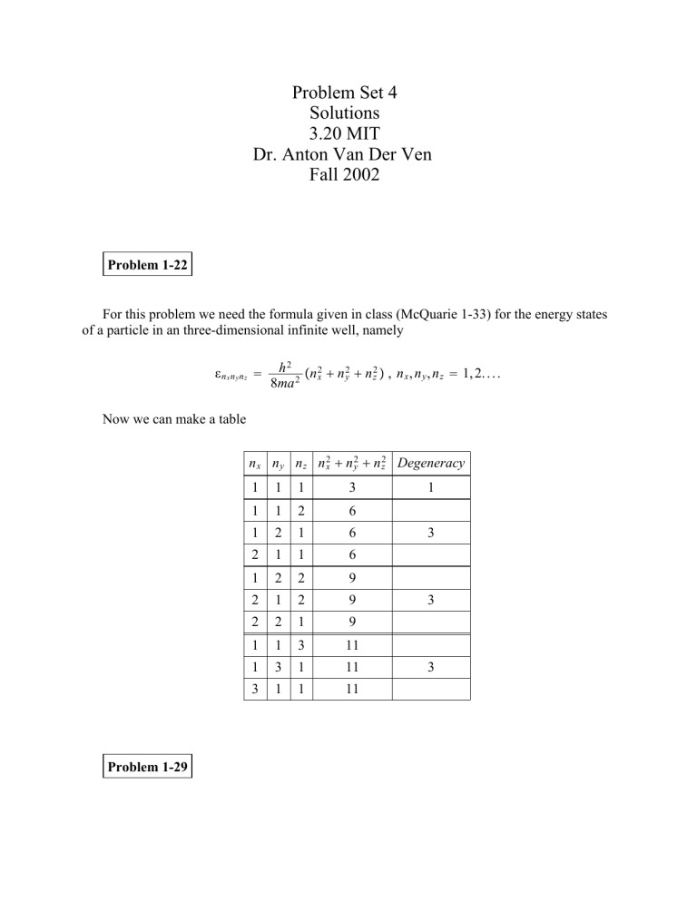
Problem Set 4
Solutions
3.20 MIT
Dr. Anton Van Der Ven
Fall 2002
Problem 1-22
For this problem we need the formula given in class (McQuarie 1-33) for the energy states
of a particle in an three-dimensional infinite well, namely
 nxnynz 
h 2 n 2  n 2  n 2  , n x , n y , n z  1, 2. . . .
x
y
z
8ma 2
Now we can make a table
n x n y n z n 2x  n 2y  n 2z Degeneracy
Problem 1-29
1
1
1
3
1
1
2
6
1
2
1
6
2
1
1
6
1
2
2
9
2
1
2
9
2
2
1
9
1
1
3
11
1
3
1
11
3
1
1
11
1
3
3
3
Start with the differential form for E
dE  TdS  pdV
E
V
We can use a Maxwell relation on
 T S
V
T
S
V
T
S
V
T
p
from FT, V
T

p
T
V
So,
E
V
T
T
p
T
V
 p
Problem 1-41
Show that x  x  2  x 2  x 2
x  x  2  x 2  2x x  x 2  x 2  2x x  x 2  x 2  2 x  x   x 2  x 2  x 2
Problem 1-43
Here we have to plot the Gaussian px 
to see what happens as   0
1
 2
exp 
x x  2
2 2
for several values of 
As   0, the function becomes sharper and sharper (remember the area under the curve is
contrained to be 1, as we will see in problem 1-44a). Thus, the Gaussian approaches a delta
function.
Problem 1-44
Gaussian distribution is
px 
(a) show 


pxdx  1

 
Let
2
1 exp  x  x 
2 2
 2
2
1 exp  x  x 
2 2
 2
dx
u  x  x , then du 
2
dx
2
So we now have

 
1 expu 2 du

And using standard integral tables or the math software, it can be show that this integral is
equal to 1.
(b) n th central moment for n  0, 1, 2, and 3
For n  0
x  x  0  1
see part a
For n  1
x  x  


  x  x   pxdx   
x  x 
x  x  2
exp 
2 2
 2
dx
Let
u  x  x , then du 
2
dx
2
Then
x  x  
1


  u  expu 2 du 
1

0
  u  expu 2 du 
1


 0 u  expu 2 du
I
II
For I let v  u and dv  du. Then

0
I 1

1

u  expu 2 du 

 0 v  expv 2 dv  II
Thus,
1


  u  expu 2 du  0
For n  2
x  x  2 
Let

 
x  x   pxdx 

 
x  x  2
x  x  2
exp 
2 2
 2
dx
u  x  x , then du 
2
3
x  x  
1


  2 2 u 2 expu 2 du 
dx
2
2 2


  u 2 expu 2 du
Now lets take a crack at this integral....

  u 2 expu 2 du
We have to do this by parts. Remembering how to do that....
yx   y  x  yx 


  y  x  yx     yx 
For our case, let
y   2u expu 2 du and x  u
2
y  expu 2  and x    1
2
So,

  u 2 expu 2 du 
u expu 2 
2




 
1
2
0

expu 2 

2
Which leaves us with,
x  x  2   2
For n  3
3
x  x  

  x  x 
3
 pxdx 

 
x  x  3
x  x  2
exp 
2 2
 2
dx
As before, let
u  x  x , then du 
2
dx
2
Then,
3
2
x  x   2 

  u 3 expu 2 
2
Since e u is a symmetric function around the origin and u 3 is an antisymmetric
function around the origin, the integral of the product of the
two functions is zero.
3
x  x   0
1
0  2
(c) lim px  lim
0
exp 
x x  2
2 2
The delta function is defined as
 x  x , the delta function


  x  a  xdx  a and   xdx  1
So lets see if this works for our case
lim 
0
Let u 
xa
 2
and du 


1 exp  x  a
2 2
 2
2
 xdx
dx
 2
lim 1
0


  expu 2   
 2 a
Since   0
1


  expu 2   a 
a


  expu 2  a

Problem 1-49
Maximize
WN 1 , N 2 , . . . . N m  
N!
m
Nj!
 j1
under the contraints that  N j  N and  E j N j  .
Since the natural log is a monotonic function, we can maximize lnW.
M  ln WN 1 , N 2 , . . . . N m   ln
Using Sterling approximation, this can be written as
N!
m
Nj!
 j1
N ln N  N   N j ln N j   N j
j
j
But the maximization must be constrained therefore we intoduce Lagrange multipliers
M  N ln N  N   N j ln N j  N j 
j
j
 Nj  N

 EjNj  
N
Remembering  N j  N and taking the derivative of M with respect to N j
M
N j
  ln N j  1    E j  0
 ln N j  1    E j
ln N j     E j , with    1  
N j  exp   expE j 
Problem 1-50
We want to show that the maximum of
WN 1 , N 2 , . . . N m  
N!
m
 Nj!
j1
occurs for N 1  N 2  N s    
N
s
Maximize
M  ln W  N ln N  N   N j ln N j   N j
subject to the constraint  N j  N. So we must use Lagrange multipliers:
M  N ln N  N   N j ln N j   N j  
 Nj  N
M   ln N  1    0
j
N j
ln N j  1    N j  exp1  
But now we must determine 
s
s
j1
j1
 N j   exp1    S exp1    N  exp1   
So
Nj 
N
s
N
s
Problem 1-51
Here we use Lagrange multipliers again with the constraint  j P j  1.
N
M    P j ln P j  
j1
N
 Pj  1
j1
Maximize
M
P j
  ln P j  1    0
P j  exp1  
Determine 
N
 P j  N exp1    1
j1
exp1    1
N
Thus
Pj 
1
N
Problem 2-1
From stat mech we get
E
V
And from thermo we have
N,

p

 p
N,V
E
V
N,T
T
p
T
N,V
 p
To show why   cont  T lets see what happens if we let   T where  is a constant
E
V
N,
 T
p
T
 p
N,V
or
E
V
N,T
but from a Maxwell relation we know
E
V
T
p
T
N,T
p
T
N,V

S
V
 T S
V
N,T
N,V
 p
N,T
and we can write
 p
dE  TdS  PdV
This statement violates the second law of thermodynamics because it implies that
Q
Q  TdS  T  dS
Problem 2-2
Given
n!
n!n  n 1 !
n 
is n 1  n 1 ?
 n 1 is the value of n 1 that maximizes n. From problem 1-50, we know that
n 1  n2 .
 n 1 is given by
n
 n1
n1 
n 1 0
n

n 1 0
n!
n 1 !nn 1 !
n!
n 1 !nn 1 !
We also know that (given in the problem):
n
y  1  x n 
 xn
1
n 1 0
n!
n 1 !n  n 1 !
If we take the derivative of y with respect to x we get
n

y  n1  x
n1

 n1xn
n 1 0
11
n!
n 1 !n  n 1 !
If we let x  1:
n
n2
n1

 n1
n 1 0
Furthermore,
n!
n 1 !n  n 1 !
2-2-1
n

2n 
n!
n 1 !n  n 1 !
n 1 0
So if we put this all together back in (2-2-1) we get
n
 n1
n1 
n!
n 1 !nn 1 !
n 1 0
n

n1
 n2 n  n  n 1
2
2
n!
n 1 !nn 1 !
n 1 0
n 1  n 1
Problem 2-5
Show that S  k  P j ln P j
We have the following three relations already
S  kT
 ln Q
T
N,V
exp
E j
kT
Pj 
 k ln Q
Q
and
Q
 exp
j
E j
kT
Starting with S we can write
Q
 k ln Q  kT
S  kT
Q
Q T
S k
Q
S k
Q

 ln
j
j
Ej
kT
exp

j
exp
E j
kT
Ej
kT 2
exp
E j
kT
E j
kT
 k ln Q
exp
E j
kT
 k ln Q
 k ln Q
E j
kT
exp
E j
S  k  ln exp
kT
j
Q
k ln Q
P j
Since  P j  1
S  k  P j  ln exp
j
E j
kT
 k ln Q
j
E j
kT
S  k  P j  ln exp
j
 k  P j  ln
j
1
Q
E j
kT
exp
S  k  P j ln
 Pj
Q
j
S  k  j P j ln P j
Problem 2-8
Q


 E j expE j 
j
 E j expE j 
E 
j

Q
E 

Q

Q

 ln Q

 ln Q

Problem 2-10
First derive E  kT 2
 ln Q
T
N,V
starting from the result of problem 2-8, namely
E 
 ln Q

From the chain rule
 ln Q
T
E 
We know  
1
kT
so
T

 kT 2 , thus
 ln Q
T
E  kT 2
 ln Q
T
We can check this by taking kT 2
kT 2
 ln Q
T
kT
N,V
Q
T
 kT 2
N,V

2 T
N,V
T

N,V
Q
E
 exp  kTj
.
 kT

Q
N,V

2 T
E
 exp  kTj
N,V
Q
E
 exp  kTj
Q

Ej
kT 2
The kT 2 cancels and we are left with
kT
2
 ln Q
T
N,V

E
 E j exp  kTj
Q
definition of E
So we have shown again that indeed E  kT 2
 ln Q
T
.
Now for the relation involving p
p 
 p j exp 
Q
Ej
kT

 
E j
V
exp 
Ej
kT
Q
p 
kT
Q
V
Q
 kT
 ln Q
V

kT V

E
 exp  kTj
j
N,T
Q
N,T
Problem 2-11
Starting with F  kT ln Q (Remember F  A
S   F
T
S  kT
 ln Q
T
V,N
p   F
V
p  kT
 ln Q
V
V,N
 k ln Q
Eqn. 2-33
T,N
Eqn. 2-32
T,N
F  E  TS  E  F  TS
E  kT ln Q  T  kT
E  kT 2
 ln Q
T
 ln Q
T
V,N
 k ln Q
Eqn. 2-31
V,N
Problem 2-13
E
For a particle confined to a cube of length a we are asked to show p j  23 Vj . We can start
with the equation for the energy states of a particle in an three-dimensional infinite well,
namely
Ej 
h 2 n 2  n 2  n 2  , n x , n y , n z  1, 2. . . .
x
y
z
8ma 2
1
Remembering that a 3  V or a  V 3 we can write E j in terms of V
2
3
2
E j  h V n 2x  n 2y  n 2z 
8m
E j
pj  
V
5
2
3
3
2
2
 2 h V n 2x  n 2y  n 2z   2  1  h V n 2x  n 2y  n 2z 
8m
3 8m
3 V
Ej
So we have
2 Ej
3 V
pj 
and taking the ensemble average gives us
p  2 E
3 V
Problem 2-14
3N
2
2mkT
h2
QN, V, T  1
N!
VN
For p ,
 ln Q
V
p  kT
ln Q  ln
T.N
 3N ln 2mkT
2
h2
p  kTN
V
1
N!
 N ln V
Now for E
E  kT
2
 ln Q
T
N,V
 kT
2
3N
2
2mk
h2
2mkT
h2
E  3N kT
2
Ideal gas equation of state is obtained when Q  fTV N  ln Q  ln fT  N ln V
p  kT
 ln Q
V
T.N
 kT
ln fT
V
p 
NkT
V
 kT
T,N
N ln V
V
Problem 2-15
We are given Q as
Q
substituting in  
3N
h
2kT
exp h
kT
exp
1
exp U o
kT
h
k
Q
3N
exp 

2T
1  exp

T

exp U o
kT
To find c v we need to use the following two relations
E  kT 2
 ln Q
T
cv 
N,V
E
T
Using your favorite math package (Maple), we can get E as
E
1
2
Uo
e  kT 3Nk e
Uo
kT
 12Nk e
U o  k
kT
 9Nk e
2  kU o
kT

1  e T
 2U o e
2
and c v as
cv 
E
T

3
Now we can take the lim c v and we find that
T
kN 2 e T

T 2 1  e T
2
Uo
kT
 4U o e
U o  k
kT
 2U o e
2  kU o
kT

k 2 e T N
lim 3
T
T
2
1  e

T
2
 3Nk