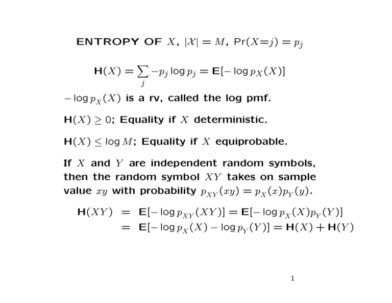
ENTROPY OF X, |X | = M , Pr(X=j) = pj
H(X) =
�
−pj log pj = E[− log pX (X)]
j
− log pX (X) is a rv, called the log pmf.
H(X) ≥ 0; Equality if X deterministic.
H(X) ≤ log M ; Equality if X equiprobable.
If X and Y are independent random symbols,
then the random symbol XY takes on sample
value xy with probability pXY (xy) = pX (x)pY (y).
H(XY ) = E[− log pXY (XY )] = E[− log pX (X)pY (Y )]
= E[− log pX (X) − log pY (Y )] = H(X) + H(Y )
1
For a discrete memoryless source, a block of
n random symbols, X1, . . . , Xn, can be viewed
as a single random symbol Xn taking on the
sample value xn = x1x2 · · · xn with probability
pXn (xn) =
n
�
pX (xj )
j=1
The random symbol Xn has the entropy
H(Xn) = E[− log pXn (Xn)] = E[− log

= E
n
�

n
�
pX (Xj )]
j=1
− log pX (Xj ) = nH(X)
j=1
2
Fixed-to-variable prefix-free codes
Segment input into n-blocks Xn = X1X2 · · · Xn.
Form min-length prefix-free code for Xn.
This is called an n-to-variable-length code
H(Xn) = nH(X)
H(Xn) ≤ E[L(Xn)]min < H(Xn) + 1
E[L(X n)]min
Lmin,n =
n
bpss
H(X) ≤ Lmin,n < H(X) + 1/n
3
WEAK LAW OF LARGE NUMBERS
(WLLN)
Let Y1, Y2, . . . be sequence of rv’s with mean Y
and variance σY2 .
The sum S = Y1 + · · · + Yn has mean nY and
variance nσY2
The sample average of Y1, . . . , Yn is
S
Y + · · · + Yn
= 1
n
n
It has mean and variance
An
Y =
E[An
y] = Y ;
σY2
n
VAR[AY ] =
Note: limn→∞ VAR[S] = ∞
n
limn→∞ VAR[An
Y ] = 0.
4
Pr{|A2n
Y −Y
| < ε}�
1
�
�
�
�
��
(y)
FA2n
Y
FAnY (y)
Pr{|AnY −Y | < ε}
�
�
Y −ε Y
y
Y +ε
The distribution of An
Y clusters around Y , clus­
tering more closely as n → ∞.
σY2
n
Chebyshev: for ε > 0, Pr{|AY − Y | ≥ ε} ≤ nε2
For any ε, δ > 0, large enough n,
Pr{|An
Y − Y | ≥ ε} ≤ δ
5
ASYMPTOTIC EQUIPARTITION
PROPERTY (AEP)
Lete X1, X2, . . . , be output from DMS.
Define log pmf as w(x) = − log pX (x).
w(x) maps source symbols into real numbers.
For each j, W (Xj ) is a rv; takes value w(x) for
Xj = x. Note that
E[W (Xj )] =
�
x
pX (x)[− log pX (x)] = H(X)
W (X1), W (X2), . . . sequence of iid rv’s.
6
For X1 = x1, X2 = x2, the outcome for W (X1) +
W (X2) is
w(x1) + w(x2) = − log pX (x1) − log pX (x2)
= − log{pX (x1)pX (x2)}
= − log{pX
1 X2
(x1x2)} = w(x1x2)
where w(x1x2) is -log pmf of event X1X2 = x1x2
W (X1X2) = W (X1) + W (X2)
X1X2 is a random symbol in its own right (takes
values x1x2). W (X1X2) is -log pmf of X1X2
Probabilities multiply, log pmf’s add.
7
For Xn = xn; xn = (x1, . . . , xn), the outcome for
W (X1) + · · · + W (Xn) is
�
n
�
n
n)
w(x
)
=
−
log
p
(x
)
=
−
log
p
(
x
n
j
j
X
X
j=1
j=1
Sample average of log pmf’s is
− log pXn (Xn)
W (X1) + · · · W (Xn)
n
=
SW =
n
WLLN applies and is
n
�
�
�
2
�
σW
� n
�
Pr
�
A
W − E[W (X)] �
≥ ε ≤
2
nε
�
�
�
�
2
� − log p (Xn)
�
σW
�
�
Xn
Pr
�
− H(X)
� ≥ ε ≤ 2 .
�
�
n
nε
8
Define typical set as
�
�
�
� − log p (xn)
�
�
Xn
− H(X)
� < ε xn :
��
�
�
n
�
Tεn =
Pr{Tε2n} �
1
�
�
�
�
FWY2n (w)
FWYn (w)
��
Pr{Tεn}
�
�
H−ε H
w
H+ε
As n → ∞, typical set approaches probability 1:
2
σ
Pr(Xn ∈ Tεn) ≥ 1 − W2
nε
9
We can also express Tεn as
�
�
Tεn = xn : n(H(X)−ε) < − log pXn (xn) < n(H(X)+ε)
�
�
Tεn = xn : 2−n(H(X)+ε) < pXn (xn) < 2−n(H(X)−ε) .
Typical elements are approximately equiprob­
able in the strange sense above.
The complementary, atypical set of strings,
satisfy
2
σW
n
c
Pr[(Tε ) ] ≤ 2
nε
For any ε, δ > 0, large enough n, Pr[(Tεn)c] < δ.
10
For all xn ∈ Tεn, pXn (xn) > 2−n[H(X)+ε].
1≥
�
xn∈Tεn
pXn (xn) > |Tεn| 2−n[H(X)+ε]
|Tεn| < 2n[H(X)+ε]
1−δ ≤
�
xn∈Tεn
pXn (xn) < |Tεn|2−n[H(X)−ε]
|Tεn| > (1 − δ)2n[H(X)−ε]
Summary: Pr[(Tεn)c] ≈ 0,
pXn (xn) ≈ 2−nH(X)
|Tεn| ≈ 2nH(X),
for xn ∈ Tεn.
11
EXAMPLE
Consider binary DMS with Pr[X=1] = p1 < 1/2.
H(X) = −p1 log p1 − p0 log(p0)
Consider a string xn with n1 ones and n0 zeros.
n
n
pXn (xn) = p11 p00
− log pXn (xn)
n1
n0
= − log p1 −
log p0
n
n
n
The typical set Tεn is the set of strings for which
− log pXn (xn)
n1
n0
= − log p1 −
log p0
H(X) ≈
n
n
n
In the typical set, n1 ≈ p1 n. For this binary
case, a string is typical if it has about the right
relative frequencies.
12
− log pXn (xn)
n0
n1
H(X) ≈
= − log p1 −
log p0
n
n
n
The probability of a typical n-tuple is about
p11 p00 = 2−nH(X).
p n p n
The number of n-tuples with p1n ones is
n!
≈ 2nH(X)
(p1n)!(p0n)!
Note that there are 2n binary strings. Most of
them are collectively very improbable.
The most probable strings have almost all ze­
ros, but there aren’t enough of them to mat­
ter.
13
Fixed-to-fixed-length source codes
For any ε, δ > 0, and any large enough n, assign
fixed length codeword to each xn ∈ Tεn.
Since |Tεn| < 2n[H(X)+ε],
1.
L ≤ H(X)+ε+ n
Pr{failure} ≤ δ.
Conversely, take L ≤ H(X) − 2ε, and n large.
Probability of failure will then be almost 1.
14
For any ε > 0, the probability of failure will be
almost 1 if L ≤ H(X)−2ε and n is large enough:
We can provide codewords for at most 2nH(X)−2εn
source n-tuples. Typical n-tuples have at most
probability 2−nH(X)+εn.
The aggregate probability of typical n-tuples
assigned codewords is at most 2−εn.
The aggregate probability of typical n-tuples
not assigned codewords is at least 1 − δ − 2−nε.
Pr{failure} > 1 − δ − 2−εn → 1
15
General model: Visualize any kind of mapping
from the sequence of source symbols X∞ into
a binary sequence Y∞.
Visualize a decoder that observes encoded bits,
one by one. For each n, let Dn be the number
of observed bits required to decode Xn (deci­
sions are final).
The rate rv, as a function of n, is Dn/n.
In order for the rate in bpss to be less than
H(X) in any meaningful sense, we require that
Dn/n be smaller than H(X) with high probabil­
ity as n → ∞.
16
Theorem: For a DMS and any coding/decoding
technique, let ε, δ > 0 be arbitrary. Then for
large enough n,
Pr{Dn ≤ n[H(X) − 2ε]} < δ + 2−εn.
Proof: For given n, let m = n[H(X) − 2ε].
Suppose that xn is decoded upon observation
of yj for some j ≤ m. Only xn can be decoded
from ym. There are only 2m source n-tuples
(and thus at most 2m typical n-tuples) that
can be decoded by time m. Previous result
applies.
17
Questions about relevance of AEP and fixedto-fixed length source codes:
1) Are there important real DMS sources? No,
but DMS model provides memory framework.
2) Are fixed-to-fixed codes at very long length
practical? No, but view length as product life­
time to interpret bpss.
3) Do fixed-to-fixed codes with rare failures
solve queueing issues? No, queueing issues
arise only with real-time sources, and discrete
sources are rarely real time.
18
MARKOV SOURCES
A finite state Markov chain is a sequence S0, S1, . . .
of discrete cv’s from a finite alphabet S where
q0(s) is a pmf on S0 and for n ≥ 1,
Q(s|s) = Pr(Sn=s|Sn−1=s)
= Pr(Sn=s|Sn−1=s, Sn−2 = sn−2 . . . , S0=s0)
for all choices of sn−2 . . . , s0, We use the states
to represent the memory in a discrete source
with memory.
19
Example: Binary source X1, X2, . . . ; Sn = (Xn−1Xn)
�
� ��
�
0; 0.9
1; 0.1
��
�
�
� ��
��
� ��
�
� �
�
� ��
� �
�
� ��
� �
�
� ��
� �
�
� ��
� �
�
� ��
�
�
��
��
� ��
�
�
00
01
1; 0.5
0; 0.5
10
��
0; 0.5
0; 0.1
1; 0.5
11
��
�
�
�
1; 0.9
Each transition from a state has a single and
distinct source letter.
Letter specifies new state, new state specifies
letter.
20
Transitions in graph imply positive probability.
A state s is accessible from state s if graph
has a path from s → s.
The period of s is gcd of path lengths from s
back to s.
A finite state Markov chain is ergodic if all
states are aperiodic and accessible from all
other states.
A Markov source X1, X2, . . . is the sequence of
labeled transitions on an ergodic Markov chain.
21
Ergodic Markov chains have steady state prob­
abilities given by
q(s) =
�
�
s ∈S
q(s)Q(s|s);
s∈S
(1)
q(s) = 1
s∈S
Steady-state probabilities are approached asymp­
totically from any starting state, i.e., for all
s, s ∈ S,
lim Pr(Sn=s|S0=s) = q(s)
n→∞
(2)
22
Coding for Markov sources
Simplest approach: use separate prefix-free
code for each prior state.
If Sn−1=s, then encode Xn with the prefix-free
code for s. The codeword lengths l(x, s) are
chosen for the pmf p(x|s).
�
2−l(x,s) ≤ 1
for each s
x
It can be chosen by Huffman algorithm and
satisfies
H[X|s] ≤ Lmin(s) < H[X|s] + 1
where
H[X|s] =
�
−P (x|s) log P (x|s)
x∈X
23
If the pmf on S0 is the steady state pmf, {q(s)},
then the chain remains in steady state.
H[X|S] ≤ Lmin < H[X|S] + 1,
where
Lmin =
H[X|S] =
�
s∈S
�
q(s)Lmin(s)
(3)
and
q(s)H[X|s]
s∈S
The encoder transmits s0 followed by codeword for x1 using code for s0.
This specifies s1 and x2 is encoded with code
for s1, etc.
This is prefix free and can be decoded instan­
taneously.
24
Conditional Entropy
H[X |S] for Markov is like H[X] for DMS.
H[X|S] =
� �
q(s)P (x|s) log
s∈S x∈X
1
P (x|s)
Note that
H[XS] =
�
q(s)P (x|s) log
s,x
1
q(s)P (x|s)
= H[S] + H[X |S]
Recall that
H[XS] ≤ H[S] + H[X]
Thus,
H[X|S] ≤ H[X]
25
Suppose we use n-to-variable-length codes for
each state.
H[S1, S2, . . . Sn|S0] = nH[X|S]
H[X1, X2, . . . Xn|S0] = nH[X|S]
By using n-to-variable length codes,
H[X|S] ≤ Lmin,n < H[X|S] + 1/n
Thus, for Markov sources, H[X|S] is asymptot­
ically achievable.
The AEP also holds for Markov sources.
L ≤ H[X|S] − ε can not be achieved, either in
expected length or fixed length, with low prob­
ability of failure.
26
MIT OpenCourseWare
http://ocw.mit.edu
6.450 Principles of Digital Communication I
Fall 2009 For information about citing these materials or our Terms of Use, visit: http://ocw.mit.edu/terms.