Massachusetts Institute of Technology
Department of Electrical Engineering and Computer Science
6.438 Algorithms for Inference
Fall 2014
22 Parameter Estimation from Partial Observa­
tions
We’ve looked at learning parameters given graph structure for directed and undirected
graphical model when all variables are observed. Today, we consider when we don’t
observe all the variables, focusing just on parameter estimation. A key issue we’ll
face is that parameters get coupled, complicating the estimation process.
22.1
Latent variables
There are numerous examples where we only observe variables partially and are re­
quired to learn the parameters associated with entire graphical model. For example,
consider a classification task such as determining whether an email received is spam
or ham. Unfortunately, email senders don’t actually give a label for whether the email
they sent is spam or ham. Thus, treating the label as a random variable, the label
is hidden and we want to infer what the label is given observations, which for email
classification could be features extracted from email content.
We give a sense of why latent variables could make estimation more difficult via
the following example:
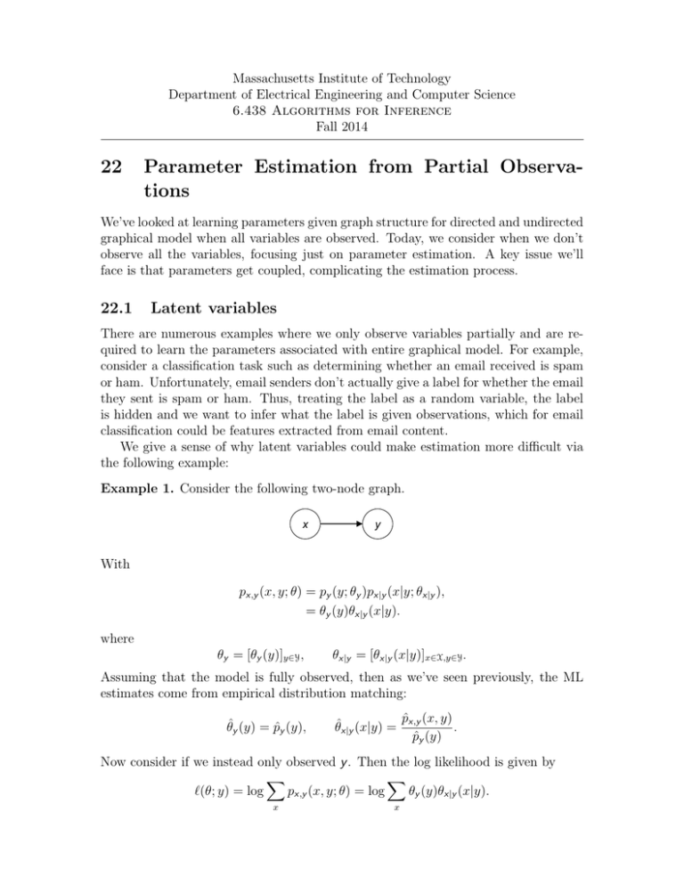
Example 1. Consider the following two-node graph.
x
y
With
px,y (x, y; θ) = py (y; θy )px|y (x|y; θx|y ),
= θy (y)θx|y (x|y).
where
θy = [θy (y)]y∈Y ,
θx|y = [θx|y (x|y)]x∈X,y∈Y .
Assuming that the model is fully observed, then as we’ve seen previously, the ML
estimates come from empirical distribution matching:
θˆy (y) = p̂y (y),
p̂x,y (x, y)
θˆx|y (x|y) =
.
p̂y (y)
Now consider if we instead only observed y . Then the log likelihood is given by
�
�
θy (y)θx|y (x|y).
�(θ; y) = log
px,y (x, y; θ) = log
x
x
for which we cannot push the log inside the summation. As a result, we cannot
separate θy from θx|y , so parameters θy and θx|y are said to “mix”. Consequently,
adjusting θy could affect θx|y .
The example above imparts the issue of parameter coupling when dealing with
latent variables. As a result, often we’re left resorting to iterative algorithms that
numerically compute ML estimates. For example, if the log likelihood is differentiable,
then we can use gradient ascent. More generally, we can view ML estimation as a
generic hill-climbing problem. But we haven’t exploited the fact that we’re dealing
with a probability distribution, which is what we’ll do next.
22.1.1
The Expectation-Maximization (EM) algorithm
Let y = (y1 , . . . , yN ) be the set of observed variables and x = (x1 , . . . , xN ' ) be the set
of latent variables, where N and N t need not be the same. We’ll refer to (y, x) as the
complete data, where we’ll assume that we know joint distribution py,x (·, ·; θ) with
parameter θ. Given observation y = y, our goal is to find the ML estimate given by
θ̂ML = arg max py (y; θ) = arg max log py (y; θ) .
θ
θ "
yv "
6i(θ;y)
We’ll refer to the log likelihood `�(θ; y) that we want to maximize as the incomplete
log likelihood, whereas we’ll call `�c (θ; y, x) = log py,x (y, x; θ) the complete log likeli­
hood, which would be the relevant log likelihood to maximize if we had observed the
complete data.
The key idea behind the EM algorithm is the following. We will introduce a
distribution q over hidden variables x that we get to choose. Notationally we’ll write
q(·|y) to indicate that we want q to depend on our (fixed) observations y. Then
`�(θ; y) = log py (y; θ)
�
X
= log
py,x (y, x; θ)
x
= log
X
�
q(x|y)
x
py,x (y, x; θ)
q(x|y)
py,x (y, x; θ)
q(x|y)
py,x (y, x; θ)
≥ Eq(·|y) log
q(x|y)
�
X
py,x (y, x; θ)
=
q(x|y) log
q(x|y)
x
= log Eq(·|y)
6 L(q, θ).
(Jensen’s inequality)
(1)
2
In particular, L(q, θ) is easier to compute since we’ve pushed the log into the sum­
mation, and we were able to do so only because we introduced distribution q and
used Jensen’s inequality and concavity of the log function. So rather than maximiz­
ing `�(θ; y), which is hard to compute, the EM algorithm will maximize lower bound
L(q, θ) by alternating between maximizing over q and then over θ:
E-step: q (i+1) = arg maxq L(q, θ(i) )
M-step: θi+1 = arg maxθ L(q (i+1) , θ)
We make a few remarks. First, in the M-step, by treating distribution q as fixed, we
are solving
py,x (y, x; θ)
arg max L(q, θ) = arg max Eq(·|y) log
θ
θ
q(x|y)
= arg max{Eq(·|y) [log py,x (y, x; θ)] − Eq(·|y) [log q(x|y)]}
θ
"
yv
"
not dependent on θ
= arg max Eq(·|y) [log py,x (y, x; θ)] .
θ
"
yv
"
(2)
6îqc (θ;y), the expected complete
log likelihood w.r.t. q(·|y)
Note that `�ˆqc (θ; y) is essentially an estimate of the incomplete log likelihood as we
are taking the expectation over hidden variables with respect to q(·|y), effectively
summing the hidden variables out but not through a marginalization. Also, note that
its the expectation of the complete log likelihood, so deriving the optimal θ will turn
out to be nearly identical to deriving an ML estimate for the complete log likelihood,
where we will fill in expected counts related to hidden variables x.
Second, the E-step can be solved explicitly. Note that if we choose q (i+1) (·|y) =
px|y (·|y; θ(i) ), then
L(px|y (·|y; θ(i) ), θ(i) ) =
�
X
=
�
X
=
�
X
px|y (x|y; θ(i) ) log
x
x
=
py,x (y, x; θ(i) )
px|y (x|y; θ(i) )
px|y (x|y; θ(i) )py (y; θ(i) )
px|y (x|y; θ ) log
px|y (x|y; θ(i) )
(i)
px|y (x|y; θ(i) ) log py (y; θ(i) )
xx
�
X
�
px|y (x|y; θ(i) ) log py (y; θ(i) )
x
"
yv
=1
(i)
= log py (y; θ )
= `�(θ(i) ; y).
3
"
So we have L(px|y (·|y; θ(i) ), θ(i) ) = `�(θ(i) ; y) while from inequality (1), we know that
`�(θ; y) ≥ L(q, θ) for all distributions q over random variable x, so it must be that
choosing q (i+1) (·|y) = px|y (·|y; θ(i) ) is optimal for solving the E-step.
By plugging the optimal choice of q from the E-step into the M-step and specifically
equation (2), we see that we can combine both steps of an EM iteration into one
update:
θ(i+1) = arg max Epx|y (x|y;θ(i) ) [log py,x (y, x; θ)]
θ
= arg max E[log py,x (y, x; θ)|y = y; θ(i) ].
(3)
θ
Hence, in the E-step, we can compute expectation E[log py,x (y, x; θ)|y = y; θ(i) ] rather
than computing out the full conditional distribution px|y (x|y; θ(i) ), and in the M-step,
we maximize this expectation with respect to θ, justifying the name of the algorithm.
We end with two properties of the algorithm. First, the sequence of parameter
estimates θ(i) produced never decreases the likelihood and will reach a local maximum.
Second, often the first few iterations will be the most useful and then the algorithm
slows down. One way to accelerate convergence after the first few iterations is to
switch to gradient ascent.
Example: Parameter estimation for hidden Markov models
Specializing to the case of HMM’s, the EM algorithm is called the Baum-Welch
algorithm (Baum et al. 1970; efficient implementation described by Welch in 2003).
Consider a homogeneous HMM given by the diagram below.
x0
x1
x2
y0
y1
y2
…
xT
…
yT
We’ll assume that xi , yi take on values in {1, 2, . . . , M }. The model parameters are
θ = {π, A, η} where:
• π is the initial state distribution (πi = px0 (i))
• A is the transition matrix (aij = pxt+1 |xt (j, i))
• η is the emission distribution (ηij = pyt |xt (j|i))
We want an ML estimate of θ given only observation y = y.
We’ll use the following data representation trick: Let xit = 1{xt = i}. Effectively,
we represent state xt ∈ {1, 2, . . . , M } as a bit-string (xt1 , xt2 , . . . , xtM ), where exactly
4
one of the xit ’s is 1 and the rest are 0. We’ll do the same for yt , letting ytj = 1{yt = j}.
This way of representing each state will prove extremely helpful in the sequel.
Before looking at the case where x is hidden, we first suppose that we observe
the complete data where we have one observation for each xi and one observation for
each yi . Then optimizing for the parameters involves maximizing the following:
log px,y (x, y; θ)
= log πx0
T
−1
g
axt ,xt+1
t=0
= log
xM
g
= log
t=0
1{x0
πi
=
M
X
�
πi 0
xi xj
aijt t+1
T −1 �
M �
M
X
X
X
�
xit xjt+1 log aij +
t=0 i=1 j=1
M
X
�
M �
M
X
X
�
T −1
X
�
i=1 j=1
t=0
i=1
6ζi
log πi +
"
1{xt =i,yt =j}
ηij
xi y j
ηij
t t
�
t=0 i=1 j=1
i=1
"yv"
�
t=0 i=1 j=1
!x T M M
�
ggg
t=0 i=1 j=1
xi0 log πi +
xi0
1{xt =i,xt+1
aij
�
!x T M M
ggg
=j}
t=0 i=1 j=1
! xT −1 M M
�
g gg
xi
i=1
=
ηxt ,yt
� xT −1 M M
!
g gg
=i}
i=1
xM
g
T
g
T X
M X
M
X
�
�
�
xit ytj
log ηij
t=0 i=1 j=1
xit xjt+1
log aij +
M X
M
T
X
�
�
X
�
yv
"
(4)
t=0
i=1 j=1
6mij
xit ytj
log ηij .
"
yv
6nij
"
Note that mij is just the number of times we see state i followed by state j in the
data. Similarly, nij is the number of times we see state i emit observation j.
M
By introducing Lagrange multipliers for constraints M
i=1 πi = 1,
j=1 aij = 1 for
M
all i, and j=1 ηij = 1 for all i followed by setting a bunch of partial derivatives to 0,
the ML estimates are given by:
π
ai = ζi ,
mij
a
aij = M
,
k=1 mik
"
yv
"
fraction of transitions
from i that go to j
nij
ηaij = M
.
k=1 nik
"
yv
"
(5)
fraction of times state i
emits observation j
We now consider the case when x is hidden, so we’ll use the EM algorithm. What we’ll
find is that our calculations above will not go to waste! Writing out the expectation
5
to be maximized in an EM iteration, i.e. equation (3), we have
Epx|y (·|y;θ(£) ) [log px,y (x, y; θ)]
"M
�
!
�
!
#
xT −1
x T
M �
M
M �
M
�
�
�
�
�
X
X
X
X
X
X
X
j
= Epx|y (·|y;θ(£) )
x0i log πi +
xti xt+1
log aij +
xti ytj log ηij
i=1
=
M
X
�
Epx|y (·|y;θ(£) ) [x0i ] log πi +
i=1 j=1
t=0
M �
M
X
X
�
xT −1
X
�
i=1
+
=
i=1
!
�
Epx|y (·|y;θ(£) ) [xti ]ytj
Epx |y (·|y;θ(£) ) [x0i ] log πi +
" 0 yv
"
log ηij
xT −1
M X
M
�
�
�
X
X
!
�
j
Epx ,x |y (·,·|y;θ(£) ) [xti xt+1
]
t t+1
"
x T
M X
M
�
X
�
X
�
log aij
t=0
i=1 j=1
ζi
+
j
Epx|y (·|y;θ(£) ) [xti xt+1
] log aij
t=0
i=1 j=1
M
X
�
!
�
t=0
i=1 j=1
x T
M �
M
X
X
X
�
�
t=0
i=1 j=1
yv
mij
"
!
�
Epx |y (·|y;θ(£) ) [xti ]ytj
log ηij .
t
t=0
i=1 j=1
"
yv
"
nij
Something magical happens: Note that using the sum-product algorithm with one
forward and one backward pass, we can compute all node marginals pxi |y (·|y; θ(i) ) and
edge marginals pxi ,xi+1 |y (·, ·|y; θ(i) ). Once we have these marginals, we can directly
j
compute all the expectations Epx |y (·|y;θ(£) ) [x0i ] and Epx ,x |y (·,·|y;θ(£) ) [xti xt+1
]; hence, we
t t+1
0
can compute all ζi , mij , and nij . Computing these expectations is precisely the Estep. As for the M-step, we can reuse our ML estimate formulas (5) from before
except using our new values of ζi , mij , and nij .
For this problem, we can actually write down the expectations needed in terms of
node and edge marginal probabilities. Using the fact that indictaor random variables
are Bernoulli, we have:
• Epx |y (·|y;θ(£) ) [xti ] = P(xt = i|y = y; θ(i) )
t
• Epx ,x
t t+1 |y
i j
(·,·|y;θ(£) ) [xt xt+1 ]
= P(xt = i, xt+1 = j|y = y; θ(i) )
Then we can simplify our ML estimates as follows:
(i+1)
π
ai
= ζ i = E px
0 |y
i
(·|y;θ) [x0 ]
6
= P(x0 = i|y = y; θ(i) ).
(6)
Next, note that the denominator of the ML estimate for a
aij can be written as
M
X
�
mik =
k=1
=
M X
T −1
X
�
�
Epx ,x
t t+1 |y
i k
(·,·|y;θ(£) ) [xt xt+1 ]
k=1 t=0
T
−1
X
�
Epx ,x
t t+1 |y
"
(·,·|y;θ(£) )
xti
t=0
=
T −1
X
�
M
X
�
#
xtk+1
k=1
Epx ,x
t t+1 |y
i
(·,·|y;θ(£) ) [xt
]
(one bit is 1 and the rest are 0 for xt+1 )
t=0
=
T −1
X
�
P(xt = i|y = y; θ(i) ).
t=0
A similar result will hold for the denominator of the ML estimate for ηaij . Thus,
PT −1
P(xt = i, xt+1 = j|y = y; θ(i) )
mij
(i+1)
a
aij
= PM
= t=0PT −1
(7)
(i) )
m
P(x
=
i|y
=
y;
θ
ik
t
k=1
t=0
PT
(i)
nij
(i+1)
t=0 P(xt = i, yt = j|y = y; θ )
ηaij
= PM
=
(8)
PT
(i)
t=0 P(xt = i|y = y; θ )
k=1 nik
In summary, each iteration of the Baum-Welch algorithm does the following:
a(i) , ηa(i) }, run the sumπ (i) , A
E-step: Given current parameter estimates θ(i) = {a
product algorithm to compute all node and edge marginals.
a(i+1) , ηa(i+1) }
a(i+1) , A
M-step: Using node and edge marginals, compute θ(i+1) = {π
using equations (6), (7), and (8).
For the E-step, if we use the α-β forward-backward algorithm, edge marginals can be
recovered using the following equation:
P(xt = xt , xt+1 = xt+1 |y = y)
∝ mt−1→t (xt ) φt (xt ) ψt,t+1 (xt , xt+1 ) φt+1 (xt+1 ) mt+2→t+1 (xt+1 )
" yv " "
yv
" " yv "
p(yt |xt )
p(yt+1 |xt+1 )
p(xt+1 |xt )
= mt−1→t (xt )p(yt |xt )p(xt+1 |xt )p(yt+1 |xt+1 )mt+2→t+1 (xt+1 )
"
#
�
X
=
αt−1 (xt−1 )p(xt |xt−1 ) p(yt |xt )p(xt+1 |xt )p(yt+1 |xt+1 )βt+1 (xt+1 )
xt−1
(recall how BP messages and α, β messages relate)
#
�
X
=
αt−1 (xt−1 )p(xt |xt−1 )p(yt |xt ) p(xt+1 |xt )p(yt+1 |xt+1 )βt+1 (xt+1 )
"
xt−1
= αt (xt )p(xt+1 |xt )p(yt+1 |xt+1 )βt+1 (xt+1 ).
7
Hence, edge marginals at iteration `� are of the form:
(i) (i)
P(xt = i, xt+1 = j|y = y; θ(i) ) ∝ αt (i)a
aij ηajyt+1 βt+1 (j).
(9)
We end our discussion of Baum-Welch with some key takeaways. First, note the
interplay between inference and modeling: In the E-step, we’re doing inference given
our previous parameter estimates to obtain quantities that help us improve parameter
estimates in the M-step.
Second, we were able to recycle our ML estimation calculations from the fully
observed case. What we ended up introducing are essentially “soft-counts,” e.g., the
new mij is the expected number of times we see state i followed by state j.
Third, by linearity of expectation, the expected log likelihood for the HMM only
ended up depending on expectations of nodes and edges, and as a result, we only
needed to compute the node and edge marginals of distribution q (i+1) = px|y (·|y; θ(i) ).
We never needed to compute out the full joint distribution px|y (·|y; θ(i) )!
8
MIT OpenCourseWare
http://ocw.mit.edu
6.438 Algorithms for Inference
Fall 2014
For information about citing these materials or our Terms of Use, visit: http://ocw.mit.edu/terms.