Massachusetts Institute of Technology
Department of Electrical Engineering and Computer Science
6.438 Algorithms For Inference
Fall 2014
Problem Set 6
Issued: Tuesday, October 28, 2014
Due: Thursday, November 13, 2014
Suggested Reading: Lecture notes 12–16
Problem 6.1
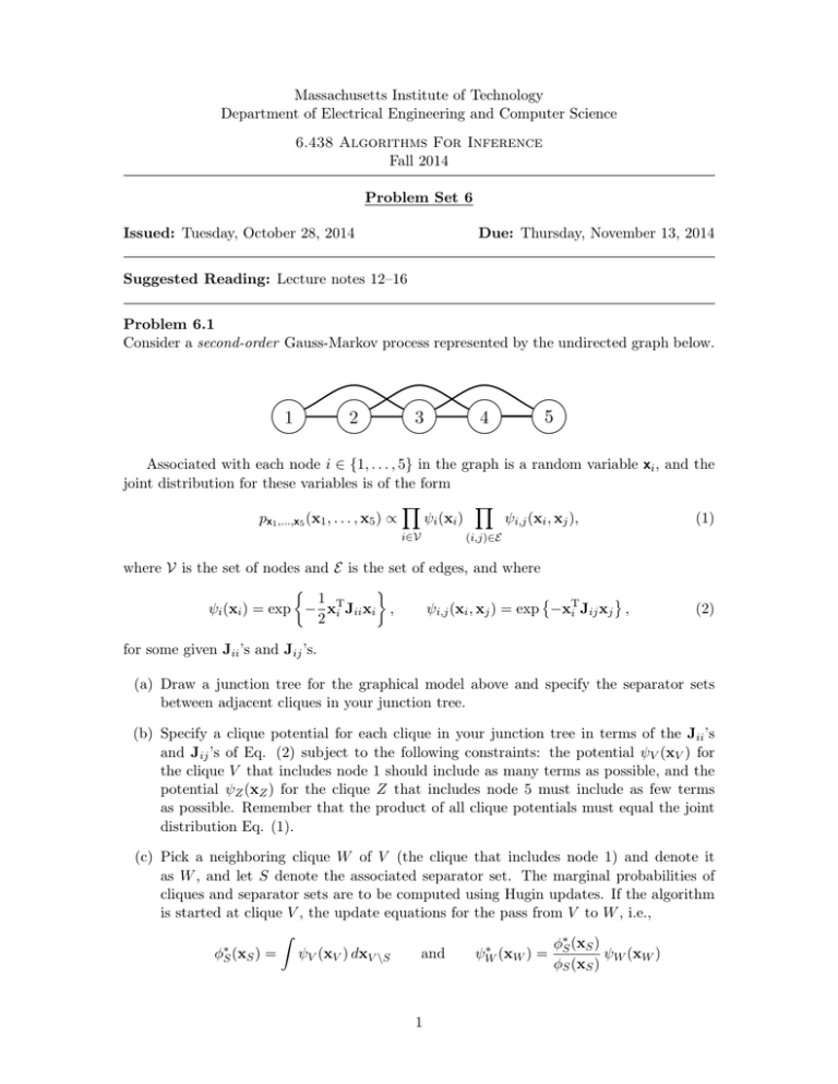
Consider a second-order Gauss-Markov process represented by the undirected graph below.
Associated with each node i ∈ {1, . . . , 5} in the graph is a random variable xi , and the
joint distribution for these variables is of the form
px1 ,...,x5 (x1 , . . . , x5 ) ∝
ψi (xi )
i∈V
ψi,j (xi , xj ),
(1)
(i,j)∈E
where V is the set of nodes and E is the set of edges, and where
�
�
1 T
ψi,j (xi , xj ) = exp −xiT Jij xj ,
ψi (xi ) = exp − xi Jii xi ,
2
(2)
for some given Jii ’s and Jij ’s.
(a) Draw a junction tree for the graphical model above and specify the separator sets
between adjacent cliques in your junction tree.
(b) Specify a clique potential for each clique in your junction tree in terms of the Jii ’s
and Jij ’s of Eq. (2) subject to the following constraints: the potential ψV (xV ) for
the clique V that includes node 1 should include as many terms as possible, and the
potential ψZ (xZ ) for the clique Z that includes node 5 must include as few terms
as possible. Remember that the product of all clique potentials must equal the joint
distribution Eq. (1).
(c) Pick a neighboring clique W of V (the clique that includes node 1) and denote it
as W , and let S denote the associated separator set. The marginal probabilities of
cliques and separator sets are to be computed using Hugin updates. If the algorithm
is started at clique V , the update equations for the pass from V to W , i.e.,
φS∗(xS ) =
ψV (xV ) dxV \S
and
1
∗
ψW
(xW ) =
φ∗S (xS )
ψW (xW )
φS (xS )
with φS (xS ) ≡ 1, can be expressed in the form
�
�
�
�
1 T ∗
1 T ∗
∗
∗
φS (xS ) = exp − xS JS xS
and
ψW (xW ) = exp − xW JW xW .
2
2
Express J∗S and J∗W in terms of the Jii ’s and Jij ’s.
Hint: You may find useful the identities
N −1 (x; ha , Ja )N −1 (x; hb , Jb ) ∝ N −1 (x; ha + hb , Ja + Jb )
and
Z
N −1
xa
h
J
Jab
; a , aa
xb
hb
Jba Jbb
dxb
−1
∝ N −1 (xa ; ha − Jab J−1
bb hb , Jaa − Jab Jbb Jba ),
when
N
−1
�
�
1 T
T
(x; h, J) ∝ exp h x − x Jx .
2
(d) Suppose that we have completed all Hugin updates and have the resulting adjusted
potentials at all (maximal) cliques and separator sets in the junction tree. Now we
observe x3 = x3 . At which cliques C can we compute pxi |x3 (xi |x3 ), where i ∈ C, from
the results of the preceding Hugin algorithm, without any further Hugin updates or
other subsequent communication between the (maximal) cliques?
Does your answer change if, instead of observering x3 , we observe x5 = x5 and seek
marginals conditioned on this observation? Explain.
Problem 6.2
For each of the graphs in Figure 1, construct a junction tree by first triangulating and then
applying a greedy algorithm. You should write each step of the greedy algorithm.
Problem 6.3
As discussed in lecture, loopy belief propagation on general (loopy) graphs is neither guar­
anteed to converge nor, when it does converge, guaranteed to yield correct marginals. In
this problem, we’ll consider an example of such phenomena on a highly symmetric graphical
model.
An Ising model on a vector of binary variables x, with each xi ∈ {+1, −1}, with param­
eter vector θ is described by
⎧
⎫
⎨�
⎬
�
θij xi xj
p(x; θ) ∝ exp
θi xi +
⎩
⎭
i∈V
(i,j)∈E
for a graph (V, E).
For this problem, we’ll consider an Ising model with ∀i ∈ V θi = 0 and ∀(i, j) ∈ E θij =
γ > 0 on a toroidal grid graph, as shown in Figure 2.
2
1
3
4
2
5
6
3
5
4
1
8
7
8
6
9
2
7
10
(a)
(b)
Figure 1
(a) Show that the single node marginal distributions are uniform for all values of γ (i.e.
Pr [xi = +1] = Pr [xi = −1] = 12 ).
(b) Implement the loopy belief propagation (sum-product) algorithm for the model.
Note that because of the symmetry introduced to make the problem easy to analyze,
our usual initialization procedure (setting all the messages to be identically 1) will
actually start the algorithm at a fixed point for any γ. (You can check that the allones messages are always fixed points of the update formula for any γ.) However,
such a fixed point may not be interesting because it may be unstable, meaning that if
our messages weren’t initialized to be exactly uniform but instead initialized within a
small neighborhood of the uniform messages, then the message updates would trend
away from the uniform fixed point. Unstable fixed points are uninteresting because
loopy BP would not find these fixed points unless initialized exactly at them, which for
general models (without so many symmetries) would not happen for any initialization
procedure. Instead of initializing the messages to be identically 1, set their
values to be near 1 but perturbed by uniformly random noise on [−0.01 0.01].
Random initialization is another standard initialization procedure, and allows us to
break the symmetry in this problem and thus only examine stable fixed points of the
loopy BP algorithm. You can check that random message initialization would also
provide correct results for BP on trees using synchronous parallel updates, but note
that the initialization of loopy BP messages will affect which fixed point is reached (if
any).
Run your implementation for various values of γ ∈ (0, 1). Find the smallest γ (up to
two decimal places) for which the algorithm converges to pseudo-marginals that are
not uniform. Provide a plot of the error in the marginals as a function of γ.
(c) Show that there exists a threshold γ ∗ > 0 such that for any γ ∈ (0, γ ∗ ), if loopy BP
converges on our model, it will yield the correct (uniform) marginals. Hint: since
3
Figure 2
all nodes are symmetric, it suffices to consider a fixed-point of the message update
formula at any node.
Problem 6.4
In this exercise, you will construct an undirected graphical model for the problem of seg­
menting foreground and background in an image, and use loopy belief propagation to solve
it.
®
Load the image flower.bmp into MATLAB using imread. (The command imshow may
also come in handy.) Partial labeling of the foreground and background pixels are given in
the mask images foreground.bmp and background.bmp, respectively. In each mask, the
white pixels indicate positions of representative samples of foreground or background pixels
in the image.
Let y = {yi } be an observed color image, so each yi is a 3-vector (of RGB values
between 0 and 1) representing the pixel indexed by i. Let x = {xi }, where xi ∈ {0, 1} is a
foreground(1)/background(0) labeling of the image at pixel i. Let us say the probabilistic
model for x and y given by their joint distribution can be factored in the form
p(x, y) =
Y
1 Y
ψ(xi , yi )
ψ(xj , xk )
Z
i
(j,k)∈E
where E is the set of all pairs of adjacent pixels in the same row or column.
Suppose that we choose
�
0.9, if xj = xk
ψ(xj , xk ) =
0.1, if xj 6=
� xk
This encourages neighboring pixels to have the same label — a reasonable assumption.
4
Suppose further that we use a simple model for the conditional distribution p(yi |xi ):
1
1
T −1
p(yi |xi = α) ∝
exp − (yi − µα ) Λα (yi − µα ) + E
2
(2π)3/2 (det Λα )1/2
for yi ∈ [0, 1]3 . That is, the distribution of color pixel values over the same type of image
region is a modified Gaussian distribution, where E accounts for outliers. Set E = 0.01 in
this problem.
(a) Sketch and label the undirected graph with respect to which the distribution p(x, y)
is Markov. What are the potential functions ψ(xi , yi )?
(b) Compute µα , Λα from the labeled masks by finding the sample mean and covariance
of the RGB values of those pixels for which the label xi = α is known.
(c) We want to run the sum-product algorithm on the graph iteratively to find (approxi­
mately) the marginal distribution p(xi |y) at every i.
Write the local message update rule for passing the message mj→k (xk ) from xj to xk ,
in terms of the messages from the other neighbors of xj , the potential functions, and
some arbitrary scaling constant.
Then write the final belief update rule on xi , that is, the marginal computation in
terms of the messages from all neighbors of xi , the potential functions, and some
arbitrary scaling constant.
(d) Implement the sum-product algorithm for this problem. There are four directional
messages: down, up, left, and right, coming into and out of each xi (except at the
boundaries). Use a parallel update schedule, so all messages at all xi are updated
at once. Run for 30 iterations (or you can state and use some other reasonable
termination criterion). You should renormalize the messages after each iteration to
avoid overflow/underflow problems.
After the marginal distributions at the pixels are estimated, visualize their expectation
(that would be the BLS estimates of xi based on y if the inference were exact). Where
are the beliefs “weak”? Where did the loopy belief propagation converge first and
last?
(e) (Practice) Convert the graph in this problem to a factor graph and write the belief
propagation messages passed between variable nodes and factor nodes.
Problem 6.5
Consider a very simple digital communication system. One of a finite number of equallylikely, length-n binary sequences (referred to as codewords) is sent by a transmitter. The
receiver obtains a corrupted version of the sent codeword. Specifically, some subset of
the elements in the codeword are erased. Moreover, the erasures are independent, and
identically distributed within a codeword, and independent of the codeword. A decoder
attempts to reconstruct the sent codeword from the un-erased elements and their locations.
5
n-element
codeword
received
sequence
channel
decoder
(codeword recovery)
(corruption)
codeword
In this problem, n = 7 and the codewords (x1 , x2 , ..., x7 ) have distribution
px1 ,x2 ,...,x7 (x1 , x2 , ..., x7 ) =
1
δ(x1 ⊕x2 ⊕x4 ⊕x5 ) δ(x1 ⊕x3 ⊕x4 ⊕x6 ) δ(x2 ⊕x3 ⊕x4 ⊕x7 ), (3)
Z
where the xi are each 0 or 1, ⊕ is addition modulo-2 (i.e., XOR), and where δ(x) = 1 when
x = 0 and is 0 otherwise.
�
1, if x = 0
δ(x) =
0, otherwise.
The (minimal) factor graph expressing the relationship between the 7 codeword symbols is
as follows:
x5
a
x1
x2
x4
b
x6
c
x3
x7
(a) Draw the undirected graph with the minimum number of edges that expresses the
relationship between the 7 codeword symbols.
(b) Determine the partition function Z in (3).
(c) If the received sequence is (0, ?, ?, 1, 0, ?, 0) where “?” denotes an erased symbol,
determine the codeword that was sent. Give an example of a received sequence with
3 erasures from which the sent codeword cannot be determined with certainty.
One method of decoding is to apply loopy belief propagation (LBP), i.e., the sum-product
algorithm in which all nodes send messages at all times. At each iteration of the algorithm,
factor nodes process all incoming messages to produce outgoing messages to variable nodes,
then, in turn, the variable nodes use these messages to produce new messages for the factor
nodes.
6
Recall that the sum-product belief propagation message-passing takes the form:
⎛
⎞
�
X
Y
⎝fs (xN (s) )
µs,i (xi ) ∝
νj,s (xj )⎠
xN (s)\i
Y
νi,s (xi ) ∝
j∈N (s)\i
µt,i (xi )
t∈N (i)\s
where µs,i (·) and νi,s (·) are the factor-to-variable and variable-to-factor messages, respec­
tively, and where N (·) denotes the neighbors of its node argument.
(d) Draw the factor graph that LBP will operate on. Include any additional variable
and/or factor nodes that are required, and indicate any modifications to factor nodes
that are required.
(e) Show that the (vector) messages in this application of LBP, when normalized so that
their largest entry is 1, take on one of only three possible values.
(f) Apply the resulting LBP algorithm to the same observed sequence (0, ?, ?, 1, 0, ?, 0)
given in part (c). Express the operation of the algorithm as follows: start by describ­
ing the initial messages; then, with each iteration, specify any factor-to-variable and
variable-to-factor messages that have changed from the previous iteration, and specify
the new values of these messages.
Remark : While this can be done by hand, coding this up to handle any length-7
sequence of 1’s, 0’s, and ?’s could be a useful exercise.
Problem 6.6
ψa
ψb
ψab
a
ψac
b
ψbc
c
ψc
Figure 3
7
(a) Consider a three-node loopy graphical model depicted in Figure 3, where the compat­
ibility functions for this model are given by the following:
ψa (0) = ψa (1) = ψb (0) = ψb (1) = ψc (0) = ψc (1) = 1
(4)
ψab (0, 0) = ψab (1, 1) = 10 ,
ψab (1, 0) = ψab (0, 1) = 1
(5)
ψac (0, 0) = ψac (1, 1) = 10 ,
ψac (1, 0) = ψac (0, 1) = 1
(6)
ψbc (0, 0) = ψbc (1, 1) = 10 ,
ψbc (1, 0) = ψbc (0, 1) = 1
(7)
(i) Compute the max-marginals at each of the three nodes. You should see that
there is a non-unique maximum for each of these.
(ii) What are the configurations of values at the three nodes of this graph that are
most probable? For this simple graph, show that you can still do something
similar to what we did in Problem 5.1 using edge-max-marginals to help us
compute one of these maximizing configurations.
(b) In general when a loopy graph has non-unique optimizing configurations, the node- and
edge-max-marginals aren’t enough to allow computation of a maximum probability
configuration. In particular, show that the triangle graph above has the following
property:
There does not exist any (deterministic) algorithm which given as input the triangle
graph and the node- and edge-max-marginals, can determine a configuration1 with
maximum probability.
For simplicity, restrict yourself to finite alphabets in this problem, i.e., each node in
your graph should only take on values from a finite set, which without of loss generality
can be denoted by 0, 1, . . . , M .
Note that the algorithm does not get access to the full probability distribution, since
otherwise there is a trivial (but potentially inefficient) algorithm to solve the problem
- compute the probability for every possible configuration, and then output a config­
uration with maximum probability. Also, note that when the graph is a tree, we saw
that the max-product algorithm can solve this problem. Specifically, given the nodeand edge-max-marginals, we saw in lecture how to break ties and compute a max­
imum probability configuration. Thus, your construction shows yet another reason
why trees are easier to deal with than graphs with cycles.
Problem 6.7 (Practice)
Consider the graph, shown in Figure 4, with a single loop, where y1 , ..., y4 are observed. Let
1
There can be multiple maximizing configurations. In this case, the algorithm’s output is considered
correct as long as it outputs some maximizing configuration.
8
y4
y3
x4
x3
x1
x2
y1
y2
Figure 4
x1 , ..., x4 be discrete random variables defined over a finite alphabet {1, 2, ..., M } for some
finite M , so we can represent edge potentials ψxi xj (xi , xj ) by matrices
⎡
⎤
ψxi xj (1, 1) . . . ψxi xj (1, M )
⎥
⎢
..
..
..
Aij = ⎣
⎦
.
.
.
ψxi xj (M, 1) . . . ψxi xj (M, M )
i.e., Aij [u, v] = ψxi xj (xi = u, xj = v). Similarly, node potentials ψxi (xi ) can be represented
by diagonal matrices
⎡
⎤
ψxi (1)
0
⎥
⎢
..
Bi = ⎣
⎦
.
0
ψxi (M )
Consider running loopy belief propagation on this graph using a parallel schedule, where
each node computes the usual sum-product messages to be passed to its neighbors, as if
(k)
the graph were acyclic. Let a column vector mij of length M denote the message that xi
sends to xj on the k-th iteration. Moreover, we will use similar vector notation to denote
the marginal probabilities of interest. For example, px1 |y will denote an M -vector whose
j-th entry is px1 |y (j|y).
(1)
(4)
(a) Express the messages m12 and m41 in terms of the matrices Aij , Bi and the initial
(0)
messages mij .
(k)
(b) Let bxi denote, in M -vector notation, the estimate of the marginal for xi produced
by this instance of loopy belief propagation that xi can compute after k iterations, in
the usual way. Specifically, at node x1 , after 4n iterations, we have
(4n)
bx1
(4n)
(4n)
∝ W(m41 8 m21 )
(8)
where 8 denotes component-wise multiplication of vectors.
(4n)
(4n)
Find m41 , m21 , and the matrix W in terms of the matrices Aij , Bi , and the initial
(0)
messages mij .
9
(c) The exact marginal px1 |y depends on the Aij and Bi only through the matrix product
A14 B4 A43 B3 A32 B2 A21 B1 . Express px1 |y in this form.
In the following, assume that all potential functions and initial messages are strictly
positive.
(d) It is a well known fact that if a matrix P and a vector z both have strictly positive
entries, then
k
P
lim
z ∝ v1 {P}
k→∞ λ1 {P}
where v1 {P} denotes the positive eigenvector of P associated with its unique largest
eigenvalue λ1 {P}.
(k)
Using this fact, it follows that the estimated marginal bx1 at node x1 converges to a
steady state
(∞)
bx1 ∝ v1 {C} 8 v1 {CT }
Express C in terms of the matrices Aij and Bi .
Hint: Aij = AT
ji .
(e) Suppose x1 , ..., x4 are binary variables, then the maximum marginal assignment based
on the steady state estimate of loopy belief propagation is correct. Show this for x1 ,
(∞)
that is, if px1 |y is the true marginal and bx1 is the steady state belief, show that
(∞)
arg max px1 |y (j|y) = arg max bx1 (j) , j ∈ {1, 2}
j
j
(∞)
(∞)
where bx1 (j) is the j-th entry of bx1 .
Hint: A 2×2 matrix P with positive entries can be expressed in the form P = VΛV−1 ,
where Λ is diagonal.
Problem 6.8
Consider the undirected graphical model depicted below.
1
2
3
4
5
6
(a) Treating node 2 as the root node, draw the computation tree corresponding to the
first 4 iterations of loopy belief propagation.
10
Associated with each node i ∈ {1, . . . , 6} in the graphical model is a binary random
variable xi ∈ {0, 1}, and the joint distribution for these variables is of the form
Y
px1 ,x2 ,x3 ,x4 ,x5 ,x6 (x1 , x2 , x3 , x4 , x5 , x6 ) ∝ ψ2 (x2 ) ψ5 (x5 )
δ(xi , xj ),
(i,j)∈E
where E is the set of edges in the graph, and, for some 0 < γ < 1,
γ
1 a = b
1 − γ x2 = 0
δ(a, b) =
,
ψ2 (x2 ) =
,
ψ5 (x5 ) =
0 a �=
γ
x2 = 1
6 b
1−γ
x5 = 0
.
x5 = 1
(b) Determine the sequence of marginal probabilities of x2 obtained from loopy belief
propagation, starting with its initialization, then after each of the first four iterations.
Assume parallel message updates, i.e., that a new message is computed along each
edge at each iteration of the algorithm.
(c) Consider the messages generated by loopy belief propagation for
o this graph, with the
messages normalized so that the message from i to j satisfies xj mij (xj ) = 1 for all
(i, j) ∈ E. Suppose
α
x3 = 0
β
x1 = 0
m23 (x3 ) =
and
m21 (x1 ) =
.
1 − α x3 = 1
1 − β x1 = 1
Determine all values of α and β such that there are messages in the graph that both
(i) satisfy the belief propagation message update equations everywhere and (ii) give
the correct marginal probability at each node.
For messages satisfying (i) and (ii), with m23 (x3 ) and m21 (x1 ) as above, specify
m12 (x2 ), m52 (x2 ), and m32 (x2 ), expressing these messages in terms of α and β.
Problem 6.9 (Practice)
Consider the Gaussian graphical model depicted below. More precisely, if we let x denote the
4-dimensional vector of variables at the 4 nodes (ordered according to the node numbering
given), then x ∼ N −1 (h, J) where J has diagonal values all equal2 to 1 and non-zero offdiagonal entries as indicated in the figure (e.g., J12 = −ρ).
(a) Confirm (e.g., by checking Sylvester’s criterion) that J is a valid information matrix—
i.e., it is positive definite—if ρ = 0.39 or 0.4.
Compute the variances for each of the components (i.e., the diagonal elements of
Λ = J−1 )—you can use MATLAB to do this if you’d like.
(b) We now want to examine Loopy BP for this model, focusing on the recursions for the
information matrix parameters.
Write out these recursions in detail for this model. Implement these recursions and
try for ρ = 0.39 and ρ = 0.4. Describe the behavior that you observe.
2
We can always achieve this by scaling the components of x.
11
3
r
r
2
r
s
4
r
1
(c) Construct the computation tree for this model. Note that the effective “J”-parameters
for this model are copies of the corresponding ones for the original model (so that every
time the edge (1,2) appears in the computation tree, the corresponding J-component
is −ρ. Use MATLAB to check the positive-definiteness of these implied models on
computation trees for different depths and for our two different values of ρ. What do
you observe that would explain the result in part (b)?
12
MIT OpenCourseWare
http://ocw.mit.edu
6.438 Algorithms for Inference
Fall 2014
For information about citing these materials or our Terms of Use, visit: http://ocw.mit.edu/terms.