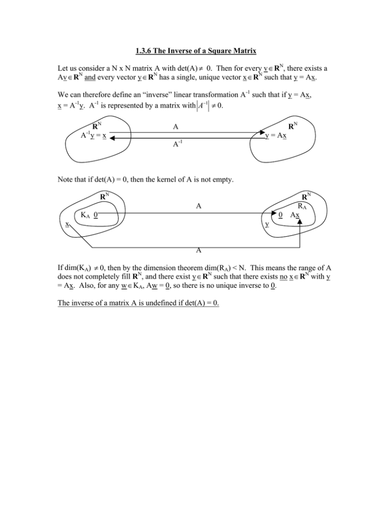
1.3.6 The Inverse of a Square Matrix
Let us consider a N x N matrix A with det(A) ≠ 0. Then for every v ∈ RN, there exists a
Av ∈ RN and every vector y ∈ RN has a single, unique vector x ∈ RN such that y = Ax.
We can therefore define an “inverse” linear transformation A-1 such that if y = Ax,
x = A-1y. A-1 is represented by a matrix with A−1 ≠ 0.
RN
A y=x
-1
RN
A
y = Ax
-1
A
Note that if det(A) = 0, then the kernel of A is not empty.
RN
A
x
KA 0
0
RN
RA
Ax
y
A
If dim(KA) ≠ 0, then by the dimension theorem dim(RA) < N. This means the range of A
does not completely fill RN, and there exist y ∈ RN such that there exists no x ∈ RN with y
= Ax. Also, for any w ∈ KA, Aw = 0, so there is no unique inverse to 0.
The inverse of a matrix A is undefined if det(A) = 0.
By the figure on page 1.3.6-1, we see that if
Y = Ax
x = A-1y
(1.3.6-1)
Then, for every x ∈ RN,
A-1Ax = A-1y = x
(1.3.6-2)
AA-1y = Ax = y
(1.3.6-3)
And for every y ∈ RN,
Therefore, is we define the identity matrix I as

1

 1



I= 
:


: 


1 
(1.3.6-4)
Sucht hat for every v ∈ RN, Iv = v (1.3.6-5)
Then
A-1A = AA-1 = I
(1.3.6-6)
Since det(I) = 1 (1.3.6-7), we have
A−1 =
1
A
(1.3.6-8)
so if
A ≠ 0, then A−1 ≠ 0.
In most applications of numerical methods, we will solve a linear system Ax=b by
Gaussian elimination, rather than calculate the inverse matrix A-1 and then obtain
x = A-1b by matrix multiplication.
But, provided for some reason we wish to calculate A-1, how is this best done?
We use the trick that when calculating the matrix product C = AB, we can write B in
terms of its column vectors b[1], b[2], ….
|
 [1]
B = b
|

| 
[2]
[N] 
b ... b 
|
| 
|
(1.3.6-9)
To obtain the column vectors of C = AB by a sequence of N matrix-vector
multiplications:
|
 [1]
C = AB = A b
|

|  |
|
|

 [1]
[N] 
[2]
[N] 
b ... b  = A b A b ... A b 

|
|  |
|
|

|
[2]
(1.3.6-10)
Therefore, let us write A-1 and I in terms of their column vectors as
|
 ~ [1]
-1
A = a

|

| 

~ [2]
~ [N]
a ... a 

|
| 

|
|
 [1]
I = e
|

|

e ... e 
|
| 
|
[2]
[N]
(1.3.6-11)
Where the kth unit vector is
0 
0 
 
: 
e[k] =  
1 
: 
 
0
We now write AA-1 = I aws
|
|  |
|
 ~ [1] ~ [2]
  ~ [1]
~ [N]
A a
a ... a  = Aa

 
|
|  |
|

 
row #k
|
|
~ [2]
Aa
|
~ [N]
... A a
|
(1.3.6-12)

 |
 = e [1]
 
 |

|
[2]
[N] 
e ... e 
|
| 
|
(1.3.6-13)
Therefore, we can obtain the N column vectors of A-1 by solving the N sets of linear
equations
~ [k]
A a = e[k]
(1.3.6-14)
If we solve these linear problems with Gaussian elimination, how many operations are
required?
For N large, the number of FLOP’s required for backward substitution is negligible
(scaling as N2) compared to the (2/3)N3 FLOP’s required to perform the elimination row
~ [k]
operations. If each linear problem A a = e[k] takes (2/3)N3 FLOP’s to solve, the total
number of FLOP’s required to obtain A-1 would seem to scale as N4. This means that
calculating A-1 would be very slow for large matrices.
But, we make an important observation:
~ [k]
Every problem A a = e[k] has the same matrix A; therefore, the sequence of row
operations performed during Gaussian elimination will be exactly the same for each
problem.
If we could somehow perform the elimination process just once, each subsequent
problem with the same matrix A would only require N2 FLOP’s of substitution to solve.
This would yield then N3 scaling for the number of FLOP’s required to obtain A-1.
The method LU decomposition allows us to perform Gaussian elimination just once when
solving a set of linear problems with the same matrix is described in section 1.4.1.